I have spent the last few weeks of Piranha development time overhauling series multipliers. In the jargon of Piranha, a series multiplier is, as the name implies, a functor that is tasked with performing the multiplication of two series.
Whereas series addition and subtraction are simple enough to be implemented in a generic fashion (and they are thus available "for free" for any series type in Piranha), series multiplication is another matter. For starters, multiplication has quadratic complexity both in time and memory, and thus it is a prime target for heavy optimisation. Secondly, the semantics of term-by-term multiplication vary quite a bit among series types. The multiplication of a monomial by another monomial, for instance, generates a single monomial, whereas the multiplication of two trigonometric monomials generates two trigonometric monomials (cf. Werner formulae). Piranha thus does not offer any generic implementation of series multiplication: whenever a new series type is introduced, a new specialisation of the series multiplier functor must be also be defined.
The polynomial multiplier is, in particular, one of the most complicated pieces of code in Piranha. Indeed, polynomials are the most basic symbolic objects that can be represented in Piranha; and, in addition to being useful and interesting per se, they are also the hierarchical building blocks of more sophisticated symbolic objects, such as Poisson series and echeloned Poisson series, which are commonly encountered in celestial mechanics. A fast, efficient polynomial multiplier is a requirement for a fast, efficient computer algebra system for celestial mechanics.
The previous iteration of the series multipliers was possibly one of the oldest parts of Piranha, dating back to circa 2011. Part of it had been renovated last year, but that had been mostly an incremental upgrade to test a few new ideas and it had actually resulted in more cruft piling over an already aging code base.
The final straw came around a month ago, when a Piranha user sent me a test case in which a medium-sized series multiplication resulted in very high memory utilisation. Without going into too much detail, this unpleasant behaviour was actually only tangentially connected to the series multipliers. I knew however that fixing this problem would involve touching multiplier code, so I took a deep breath and dove in.
The new polynomial multipliers
Conceptually, polynomial multiplication is rather trivial: multiply each monomial of the first factor by all the monomials of the second factor, and accumulate the results of these monomial-by-monomial multiplications in some data structure. Piranha uses a hash table for this purpose.
(For dense univariate polynomials, faster algorithms based on techniques such as Fourier transforms and Karatsuba multiplication exist. These methods are however unsuitable for sparse and multivariate polynomials)
The complicated part is to code an efficient implementation of this simple algorithm. One of the major difficulties is the optimisation of the memory access pattern: sparse polynomial multiplication tends to generate huge amounts of data from small operands and in a short amount of time, and it is thus very susceptible to the memory wall. This problem becomes even more challenging in a parallel multiplication algorithm, as multiple cores need to share a memory bus with limited bandwidth.
Piranha tries to address these difficulties with a series of techniques aimed at reducing the pressure on the memory system:
- the exponents of a multivariate monomial are packed into a single integer using a technique called Kronecker substitution. This allows to avoid using dynamic memory in the representation of a monomial;
- the hash table that stores the monomials avoids dynamic memory allocation for those buckets containing less than two elements. Each bucket of the table is represented by a singly linked list with inlined heads;
- Kronecker substitution is actually also a form of homomorphic hashing which allows to split the multiplication between multiple threads which can run independently without communication and without interfering with each other. It also allows to schedule the operations in a way which is friendly to the hardware prefetcher.
It should be noted that it is not always possible to use Kronecker substitution. For instance, Puiseux series require the exponents to be rationals. Even in standard polynomials, if the number of variables and/or the range of the integral exponents is large enough, it will not be possible to pack small integers into a big integer. For these cases, Piranha provides another polynomial implementation which stores monomials as vector-like objects and which uses a different implementation of the multiplication algorithm. This second implementation is less efficient than the first one, but on the flip side it is readily generalisable: much of its code is shared with the multipliers for Poisson series, divisor series and echeloned Poisson series.
Speedups in the Kronecker multiplier
The implementation of the Kronecker multiplier has not changed much from an algorithmic point of view. The only algorithmic improvement that I implemented in the new Kronecker multiplier is a form of load balancing when using multiple threads. In the old implementation, the total workload would be divided equally and upfront among the available threads. This worked fairly well in practice, but this type of static scheduling had some drawbacks:
- it assumed that the cost of a monomial multiplication would be fixed, whereas that it not necessarily the case (e.g., the cost of multiplying arbitrary-precision integral coefficients is definitely not constant - it depends on the size of each coefficient);
- it didn’t take into account the cost of managing threads: even if each thread receives the same workload, some threads will start processing earlier than other threads. The more cores are available, the more pronounced this effect becomes: the last thread will start processing data later than the first thread, and the first thread will complete its workload earlier than the first thread.
In order to provide some form of load balancing, I implemented a work stealing technique. Instead of dividing the total workload into N parts (where N == number of threads), the total workload is now divided into N * M work packages (where M is a small integral value). Each work package is associated to an atomic variable that indicates whether the work package has been consumed or not. Whenever a thread grabs a work package, it will flip the the atomic variable via an atomic compare+swap operation to signal that the work package has been consumed and does not need to be processed by another thread. This way, a thread cannot become idle if there is still work to do - it will just grab an available work package and process it.
In order to compare the performance of the old and new Kronecker multipliers, I used the following multiplication as a benchmark:
\begin{equation*}
\left(x + y + z^2 + t^3 + u^5 + 1\right)^{25}\cdot\left(u + t + z^2 + y^3 + x^5 + 1\right)^{25}
\end{equation*}
This is a rather massive sparse polynomial multiplication that results in a polynomial of circa 312 million terms, the representation of which requires around 40GB of memory. All tests were run on a Linux 64-bit machine powered by an Intel Xeon E5-2687W v3 @ 3.10GHz and 64GB of RAM. The machine has two separate processors with 10 cores each, for a total of 20 cores. This is the comparison between the new and old Kronecker multipliers:
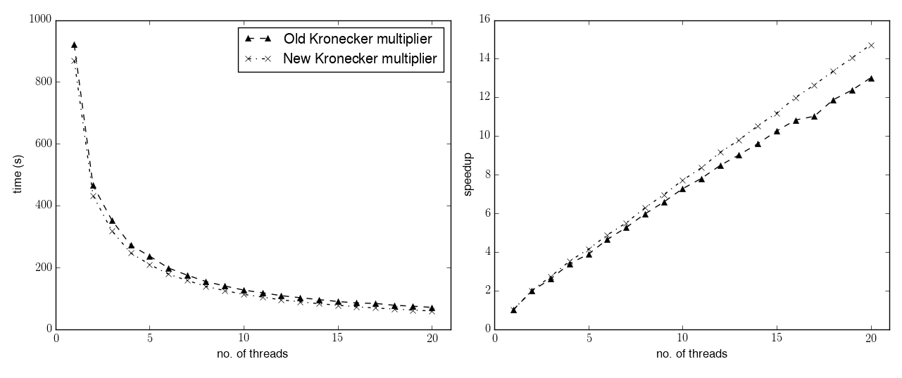
The left panel displays the runtime in seconds as a function of the number of cores used. The right panel displays the speedup (that is, the ratio between the runtime with one thread and the runtime with N threads) as a function of the number of threads.
Right off the bat, a small speedup can already be observed with a single thread. When going back refactoring old code, it often happens that in the ensuing cleanup and reorganisation of the code some moderate speedup is achieved, and this case was no exception. When the number of threads increases, the new multiplier not only maintains the speedup observed in the single-threaded scenario, but it also manages to achieve a better scaling behaviour with respect to the old multiplier. The old multiplier has a parallel speedup of 13 with 20 threads, while the new multiplier achieves a speedup of 14.7 with the same number of threads.
The speedup in this specific benchmark is not caused by the better load balancing behaviour. Indeed, for both the new and the old multiplier, the difference in runtime between the slowest and the fastest thread is around 5-6% of the runtime of the slowest thread.
The load balancing behaviour can be appreciated in this other test:
\begin{equation*}
\left(x + y + z^2 + t^3 + u^5 + 1\right)^{16}\cdot\left(u + t + z^2 + y^3 + x^5 + 1\right)^{16}
\end{equation*}
This is a smaller version of the previous test. The result in this case has a size of circa 28 million terms. Here are the performance measurements:
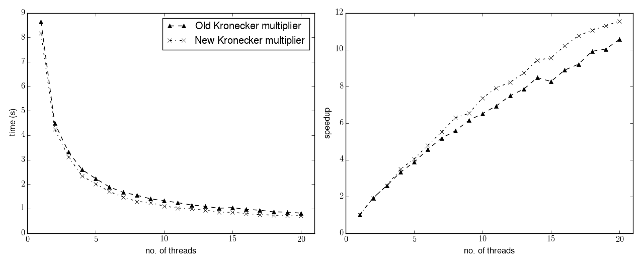
The runtime of this second test is much reduced with respect to the first one (~9 vs ~900 seconds in single-threaded mode). The scaling behaviour is more erratic and less efficient than in the first test: this is probably because when many threads are used the total runtime becomes rather short (0.7-0.8 seconds), and the overhead of setting up the parallel algorithm starts to become noticeable.
We can observe also in this test the improved behaviour of the new multiplier, both with respect to the total runtime and to the parallel scaling. The load balancing is now also more prominent: while the old multiplier has a relative difference of 20% between the runtime of the slowest and fastest threads, in the new multiplier the difference has decreased to 7%.
Speedups in the general multiplier
As explained above, when Kronecker substitution cannot be applied, another multiplication algorithm has to be adopted. This algorithm can handle not only polynomials with arbitrary exponent types (including, e.g., rational exponents), but it is also suitable - with minimal modifications - for the multiplication of other series types, including Poisson series and divisor series. Hence, the "general" moniker.
In the general multiplier, the hashing of terms loses the homomorphic property that was exploited by the Kronecker multiplier. Thus, in order to provide parallel multiplication capabilities, the old implementation would accumulate the result of the multiplication in different hash tables in parallel (one per thread), and would then perform one final merge step of all the tables at the end.
The new general multiplier, just like the Kronecker one, uses a single table shared among all the threads. In order to avoid multiple threads writing concurrently into the same memory location, each bucket is now protected by a spinlock implemented via C++11 atomic primitives.
Here are the timings for the second benchmark (the small one), where monomials are now represented as arrays of 8-bit integers:
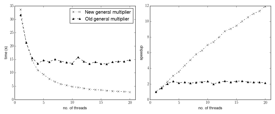
The first observation is that the change in the representation of the monomials results in the single-threaded timings increasing more than threefold with respect to the Kronecker multiplier. Secondly, the new multiplier actually shows a small decrease in performance in single-threaded mode (circa 6%) with respect to the old one. I am not completely sure why this happens. It could be that the new code is harder for the compiler to optimise (I have seen this happening before), or it could be that there really is something that can be improved in single-threaded mode. In any case, the regression is quite minor.
On the flip side, the new multiplier has a much better scaling behaviour. The old multiplier could not really scale past 3-4 threads, whereas the new implementation achieves a speedup of 12 with 20 threads - which is similar to the speedup achieved by the Kronecker multiplier. Even better, the same behaviour can be expected for all those series types which use the new general multiplier (even though I don’t have any benchmark available at the moment).
To me it was a bit surprising that such a simple strategy (i.e., one lock per bucket) could be so effective in practice. I had tried a similar approach a few years ago, but at the time I had used regular mutexes rather than spinlocks (I don’t think atomic variables had been implemented by most compilers back then) and the results had been rather appalling.
Closing remarks
I am really satisfied with the performance of the new multipliers. I have a few extra improvements and ideas in mind for the future, but for now I will go ahead and merge soon this new code into the master branch.
The new implementations of the multipliers are shorter than the old ones, so the net effect of this work was actually a decrease of the number of lines of code. Additionally, the new multipliers have better test coverage. In the end, the ratio between lines of tests and lines of source code increased from 1.61 to 1.69.
As a last bit of trivia, I should probably mention what happened to the original bugreport that triggered this work. The series multiplication test case that would use tens of gigabytes of memory and take tens of seconds to run, now uses less than 1GB of RAM and completes in around 1 second. The new multipliers played a minor part in this improvement, which is actually ascribed to a rework of series truncation. But this is material for another post.