Optimal Control of the Lotka-Volterra equations

In this tutorial we study an optimal control problem for the Lotka-Volterra equations.These famous equations are frequently used to describe the dynamics of biological systems in which two species interact: a predator (\(y\)) and a prey (\(x\)).

The dynamics considered, taken from the work of Aitziber Ibanez, is:

\[\begin{split} (1) \quad \left\{ \begin{array}{l} \dot x = p_0 x - p_1 xy - p_4 x u\\ \dot y = p_2 xy - p_3 y - p_5 y u\\ \end{array} \right. \end{split}\]

where \(p_i > 0\) and \(0 <= \vert u\vert <= 1\) is a control variable describing our hunting capabilities assumed to be proportional to the number of individuals in each of the two species.

NOTE: we used the symbols \(p_i\) for all parameters as \(p\) it is the default symbol used in heyoka.py streams, and thus it allows consistency in notation throughout the notebook.

We are interested in finding \(u(t)\) in the functional space of piecewice continuous functions such that the system is steered into a terminal state \(x_f, y_f\) in minimal time when starting from some intial condition \(x_0, y_0\).

More formally, we consider the following optimal control problem (OCP):

\[\begin{split} \begin{array}{rl} \mbox{find:} & u(t), t_f \\ \mbox{subject to (dynamics):} & \dot x = p_0 x - p_1 xy - p_4 x u\\ & \dot y = p_2 xy - p_3 y - p_5 y u\\ \mbox{subject to (boundary conditions):} & x(0) = x_0, \quad x(t_f) = x_f\\ & y(0) = y_0, \quad y(t_f) = y_f\\ & 0 <= \vert u\vert <= 1 \\ \mbox{to minimize:} & t_f \\ \end{array} \end{split}\]

To solve the above OCP we will apply Pontryagin maximum principle (PMP) maximizing \(-t_f\). We will thus eventually transform the problem above into a two-point boudary value problem (TPBVP) for an augmented set of ordinary differential equation (ODE) which we will solve using heyoka.py.

Let us start importing a few core tools:

import heyoka as hy
import numpy as np
from matplotlib import pyplot as plt

import sympy.simplify as pretty

Deriving the augmented dynamics

The straightforward application of the PMP requires the introduction of auxiliary functions \(\boldsymbol\lambda(t)\) and of a Hamiltonian which, in the case of a minimum time problem is:

\[ \mathcal H(\mathbf x, \boldsymbol\lambda, u) = \mathbf f \cdot \boldsymbol\lambda - 1 \]

where we indicated with the symbol \(\mathbf f\) the r.h.s. of the dynamics.

We define the system state, the co-states (or augmented states, essentially some form of continuous version of Lagrange multipliers) \(\lambda_x, \lambda_y\) and the dynamics:

# Define the symbolic variables x, y and th.
x, y = hy.make_vars("x", "y")

# the co-states lx, ly 
lx, ly = hy.make_vars("lambda_x", "lambda_y")

# the control
u = hy.make_vars("u")

# and the dynamics fx, fy
fx = hy.par[0]*x - hy.par[1]*x*y - x * hy.par[4] * u
fy = hy.par[2]*x*y - hy.par[3]*y - y * hy.par[5] * u

and the expression for the Hamiltonian:

# The Hamiltonian for the minimal time problem
H = fx*lx + fy*ly - 1
print("The Hamiltonian:")
pretty(H.__repr__())

The Hamiltonian:

\[\displaystyle - \lambda_{x} x \left(- p_{0} + p_{1} y + p_{4} u\right) - \lambda_{y} y \left(- p_{2} x + p_{3} + p_{5} u\right) - 1.0\]

Note how in heyoka.py expression system system parameters are indicated with the symbols \(p_i\) in the screen output.

According to the PMP the value of the control \(u\), along an optimal trajectory, is such that:

\[ u^* = \max_{u\in\mathcal U} \mathcal H(\mathbf x, \boldsymbol\lambda, u) \]

where we have introduced the space of admissible controls as the closed interval \(\mathcal U = [0,1]\). In our case we get, quite simply:

\[\begin{split} u^*(\mathbf x, \boldsymbol\lambda) = \left\{\begin{array}{ll} 1 & -(p_4 x\lambda_x+p_5 y \lambda_y) > 0 \\ 0 & -(p_4 x\lambda_x+p_5 y \lambda_y) < 0 \end{array} \right. \end{split}\]

The value of the control will then switch between the extreme values 0 and 1 whenever the switching function \(S(\mathbf x, \boldsymbol \lambda) = -(p_4 x\lambda_x+p_5 y \lambda_y)\) changes sign.

We implement two python functions to compute the switching function and the hamiltonian \(\mathcal H(\mathbf x, \boldsymbol\lambda, u^*)\):

def _switching_function(x,y,lx,ly,p):
    """The non vectorized form for the switching function
    
    Args:
        x,y,lx,ly (float): augmented system state.
        p (1-D np.array): system parameters.

    Returns:
        float: The value of the switching function.
    """
    return -(p[4]*x*lx+p[5]*y*ly)

# Vectorized version
def switching_function(x,y,lx,ly,p):
    vectorized = np.vectorize(lambda x,y,lx,ly: _switching_function(x,y,lx,ly,p))
    return vectorized(x,y,lx,ly)

# Introduce a compiled function
# for the evaluation of the Hamiltonian.
H_cf = hy.cfunc([H], vars=[x, y, lx, ly, u])

def _hamiltonian(x,y,lx,ly,p):
    sw_v = switching_function(x,y,lx,ly,p)
    u_opt = 0
    if sw_v > 0:
        u_opt = 1
    
    return H_cf([x, y, lx, ly, u_opt], pars=p[:6])[0]

# Vectorized version
def hamiltonian(x,y,lx,ly,p):
    vectorized = np.vectorize(lambda x,y,lx,ly: _hamiltonian(x,y,lx,ly,p))
    return vectorized(x,y,lx,ly)

The equations of motion in the augmented state (\(\mathbf x, \boldsymbol \lambda\)) are the Hamilton’s equations:

\[\begin{split} \begin{array}{l} \dot {\mathbf x} = \frac{\partial \mathcal H}{\partial \boldsymbol \lambda} \\ \dot {\boldsymbol \lambda} = - \frac{\partial \mathcal H}{\partial \mathbf x} \end{array} \end{split}\]

let us compute them:

# We compute the co-state equations
flx = -hy.diff(H, "x")
fly = -hy.diff(H, "y")

print("Co-state dynamics (1):")
pretty((flx).__repr__())

Co-state dynamics (1):

\[\displaystyle \lambda_{x} \left(- p_{0} + p_{1} y + p_{4} u\right) - \lambda_{y} p_{2} y\]

print("Co-state dynamics (2):")
pretty((fly).__repr__())

Co-state dynamics (2):

\[\displaystyle \lambda_{x} p_{1} x + \lambda_{y} \left(- p_{2} x + p_{3} + p_{5} u\right)\]

Putting everything together (i.e. substituting the expression for the optimal \(u^*\) found via the PMP into the augmented equations) we get:

\[\begin{split} (2) \quad \left\{ \begin{array}{l} \dot x = p_0 x - p_1 xy - p_4 x u^*\\ \dot y = p_2 xy - p_3 y - p_5 y u^*\\ \frac{d \lambda_x}{dt} = (-p_0 + p_1 y + p_4u^*) \lambda_x - \lambda_y p_2 y \\ \frac{d \lambda_y}{dt} = p_1 x \lambda_x +(-p_2 x + p_3 + p_5 u^*) \lambda_y \\ \end{array} \right. \end{split}\]

As dictated by Pontryagin’s Theorem, a necessary condition for a trajectory to be optimal is that intial values \(\boldsymbol \lambda_0\) exist such that the solution of the above ODE initial value problem (IVP) from \([\mathbf x_0, \boldsymbol \lambda_0]\) leads the system to the desired target state. Furthermore, if the final time \(t_f\) is left free \(\mathcal H_f = \mathcal H(\mathcal x_f, \boldsymbol \lambda_f) = 0\).

Formally, we seek a root of the system of (three) nonlinear equations in the (three) unknowns \(\boldsymbol \lambda_0, t_f\):

\[\begin{split} (3)\qquad \varphi(\boldsymbol \lambda_0, t_f) = \left[ \begin{array}{l} x(t_f) - x_f \\ y(t_f) - y_f \\ \mathcal H (t_f) \end{array} \right] \end{split}\]

also called shooting function as finding its root requires solving multiple times an IVP in a “clever” trial and error iterative scheme.

In the following we will be using heyoka.py to first study the uncontrolled dynamics, then to study the augmented dynamics and, finally, to define a clever, reduced, shooting function that can be easily solved by a root finder.

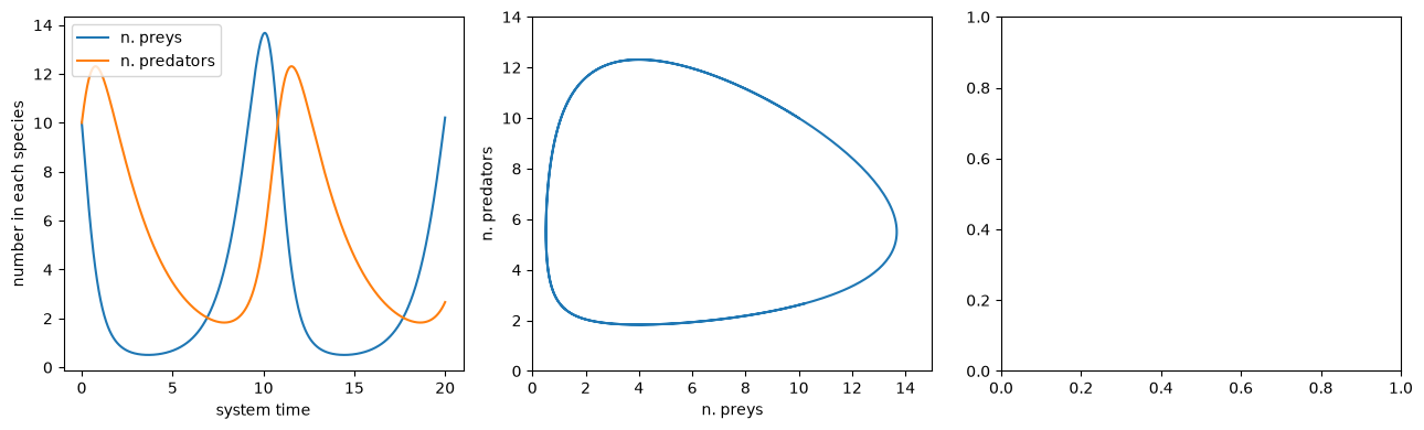
Studying the uncontrolled system

Let us see what happens in an uncontrolled case. We will consider an initial population of 10 preys with growth rates \(p_0= 1.1\), \(p_1 = 0.2\) and 10 predators with growth rates \(p_2 = 0.1\), \(p_3 = 0.4\).

We write the r.h.s. of Eq.(1). The parameters in the equations are indicated symbolically by the syntax par[i]. Their numerical value will be set later.

# Dynamics
fx_unc = hy.par[0]*x - hy.par[1]*x*y 
fy_unc = hy.par[2]*x*y - hy.par[3]*y

# System parameters
ps = [1.1, 0.2, 0.1, 0.4]

# Initial conditions
x_0, y_0 = 10., 10.

The actual EOM, in the heyoka.py syntax, can be specified as a list of tuples (variable, equation):

ode_sys_unc = [(x,fx_unc), (y, fy_unc)]

We now create the integrator object, using as initial conditions 10, 10.

ta = hy.taylor_adaptive(ode_sys_unc, state = [x_0,y_0], pars = ps)
print(ta)

C++ datatype            : double
Tolerance               : 2.220446049250313e-16
High accuracy           : false
Compact mode            : false
Taylor order            : 20
Dimension               : 2
Time                    : 0
State                   : [10, 10]
Parameters              : [1.1, 0.2, 0.1, 0.4]

We may now solve the IVP, since we want to record the state and show its trend we use the propagate_grid method which efficiently returns the system state along a predefined time grid.

t_grid = np.linspace(0,20,1000)
outcome, min_h, max_h, steps, _, sol = ta.propagate_grid(t_grid)

… and plot the solution … (note that we recorded also other quantities … but we are not really using them here)

fig, axs = plt.subplots(1,3, figsize=(13,4))
preys_unc = sol[:,0]
predators_unc = sol[:,1]

axs[0].plot(t_grid, preys_unc, label="n. preys")
axs[0].plot(t_grid, predators_unc, label="n. predators")
axs[0].legend(loc=2)
axs[0].set_xlabel("system time")
axs[0].set_ylabel("number in each species")

axs[1].plot(preys_unc, predators_unc)
axs[1].set_xlabel("n. preys")
axs[1].set_ylabel("n. predators")
axs[1].set_xlim([0,15])
axs[1].set_ylim([0,14])

plt.tight_layout() 

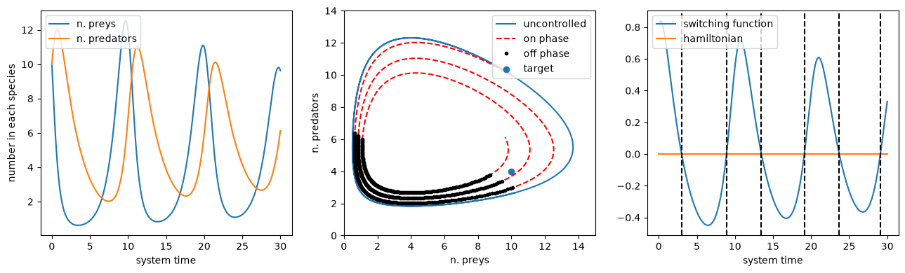
Controlling the prey-predator dynamics

We now study the augmented system of equations. This will be used later in the shooting method.

We define our ODE first:

# Dynamics
fx = hy.par[0]*x - hy.par[1]*x*y - x * hy.par[4] *  hy.par[6]
fy = hy.par[2]*x*y - hy.par[3]*y - y * hy.par[5] *  hy.par[6]
flx = (-hy.par[0] + hy.par[1]*y + hy.par[6] * hy.par[4]) * lx - hy.par[2]*ly*y
fly = hy.par[1]*x*lx + (-hy.par[2]*x + hy.par[3] + hy.par[6] * hy.par[5]) * ly
ode_sys = [(x,fx), (y, fy), (lx, flx), (ly, fly)]

# System parameters
p0,p1,p2,p3,p4,p5,p6 = ps = [1.1,0.2, 0.1,0.4,0.03,0.03, 0.]

# Target conditions
x_t, y_t = 10., 4.

# A random choice for the initial costates
lx_0, ly_0  =-1.105, -1.6274561403508774

We have added three parameters to the system. The first ones are par[4] and par[5] representing the values of \(p_4, p_5\). Then, par[6] is the value of the optimal control \(u^*\) effectively determining which one of two different systems of ODEs gets propagated. Its value is decided, as seen above, by the value of the switching function.

We now build the system of equations taking care to define in heyoka.py a terminal event detecting the change in sign of the switching function and thus changing the optimal control accordingly.

# Here we record the switching times
switch_times = []

# This callback will be called by the Taylor integrator when the switching event is detected 
def switch_callback(ta, log_times):
    if ta.pars[6]==0.:
        ta.pars[6] = 1.
    else:
        ta.pars[6]=0.
    if log_times:
        switch_times.append(ta.time)
    # Do not stop the integration
    return True
        
# The switching event
switching_event = hy.t_event(x * lx * hy.par[4] + y * ly * hy.par[5],
                             callback = lambda ta, d_sgn: switch_callback(ta, True))

# The Taylor integrator
ta = hy.taylor_adaptive(ode_sys, [x_0, y_0, lx_0, ly_0], pars = ps, t_events = [switching_event])

# We must set the initial value of the parameter par[6] representing u^* to its optimal value at t=0
ta.pars[6] = np.heaviside(switching_function(x_0,y_0,lx_0,ly_0, ps), 1.)
print(ta)

C++ datatype            : double
Tolerance               : 2.220446049250313e-16
High accuracy           : false
Compact mode            : false
Taylor order            : 20
Dimension               : 4
Time                    : 0
State                   : [10, 10, -1.105, -1.6274561403508774]
Parameters              : [1.1, 0.2, 0.1, 0.4, 0.03, 0.03, 1]
N of terminal events    : 1

We now integrate the system. The resulting trajectory will be optimal, but not respecting the requested boundary conditions, since the final time \(t_f\) and the initial values of the costates were randomly chosen.

t_grid = np.linspace(0,30,1000)
outcome, min_h, max_h, steps, _, sol = ta.propagate_grid(t_grid)

and replot the result, comparing it to the previous uncontrolled system.

fig, axs = plt.subplots(1,3, figsize=(13,4))
preys = sol[:,0]
predators = sol[:,1]
lpreys = sol[:,2]
lpredators = sol[:,3]

sf_num = switching_function(preys, predators, lpreys, lpredators, ps)
H_num = hamiltonian(preys, predators, lpreys, lpredators, ps)
mask_on = sf_num > 0
mask_off = sf_num < 0

axs[0].plot(t_grid, preys, label="n. preys")
axs[0].plot(t_grid, predators, label="n. predators")
axs[0].legend(loc=2)
axs[0].set_xlabel("system time")
axs[0].set_ylabel("number in each species")

axs[1].plot(preys_unc, predators_unc, label="uncontrolled")
axs[1].plot(preys, predators, 'r--', label = "on phase")
axs[1].plot(preys[mask_off], predators[mask_off], 'k.', label = "off phase")
axs[1].set_xlabel("n. preys")
axs[1].set_ylabel("n. predators")
axs[1].set_xlim([0,15])
axs[1].set_ylim([0,14])
axs[1].scatter([x_t], [y_t], label='target')
axs[1].legend(loc=1)

axs[2].plot(t_grid, sf_num, label="switching function")
axs[2].plot(t_grid, H_num, label="hamiltonian")
for time in switch_times:
    axs[2].axvline(x=time, color='k', linestyle='--')
axs[2].set_xlabel("system time")
axs[2].legend(loc=2)

plt.tight_layout() 

Implementing a single shooting method

Above we have produced an optimal trajectory, only not the one we looked for since we want to achieve the terminal conditions \(x_f = 10, y_f=4\) and (free time) \(H_f=0\). The choice we made for \(\lambda_{x0}\), \(\lambda_{y0}\), \(t_f\) was not a good one, we need to change it up to when Eq.(3) is actually satisfied.

In this case, to showcase the possibilities offered by heyoka.py, we will vary \(\lambda_x\), find \(\lambda_y\) from the condition \(\mathcal H_f = \mathcal H_0 = 0\) and find \(t_f\) as the time along the generated trajectory when the difference between the state and the target is minimal (a terminal event).

This reduces the free shooting parameters in Eq.(3) from three to one only: \(\lambda_x\).

The following holds (from \(\mathcal H_f = \mathcal H_0=0\)): $\( \lambda_{y0} = \frac{x\lambda_{x0}(p_0-p_1 y_0-p_4 u^*_0-1)}{y_0(-p_2x_0+p_3+p_5 u^*_0)} \)$ and it is implemented in the function below:

def find_lambda_y0(x_0,y_0,lx_0,p):
    #we assume u*=0
    ly_0 = (x_0*lx_0*(p[0]-p[1]*y_0)-1)/y_0/(-p[2]*x_0+p[3])
    if _switching_function(x_0,y_0,lx_0,ly_0,p) < 0:
        #the assumption holds
        return ly_0
    ly_0 = (x_0*lx_0*(p[0]-p[1]*y_0-p[4])-1)/y_0/(-p[2]*x_0+p[3]+p[5])
    if _switching_function(x_0,y_0,lx_0,ly_0,p) > 0:
        #the assumption holds
        return ly_0
    raise ValueError

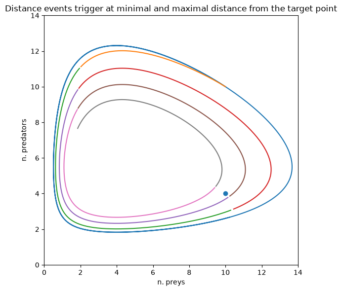
We also need to introduce a distance event triggering when the derivative of the distance is zero, hence at the maximum and minimum distance points.

def distance_callback(ta, d_sgn):
    candidates_t.append(ta.time)
    candidates_d.append((ta.state[0]-x_t)**2 + (ta.state[1]-y_t)**2)
    # Do not stop the integration
    return True

# This is the new "distance" event
distance_event = hy.t_event((x- x_t)*fx + (y-y_t)*fy, callback = distance_callback)

# We also redefine the switching event as we have no need to log the switching times (this is optional and has not real impact in this case)
switching_event_no_log = hy.t_event(x * lx * hy.par[4] + y * ly * hy.par[5],
                                    callback = lambda ta, d_sgn: switch_callback(ta, False))

Let us check that all is in order performing again the same integration and visualizing the new event triggers ….

ta = hy.taylor_adaptive(ode_sys, [x_0, y_0, lx_0, ly_0], pars=ps, t_events = [switching_event_no_log, distance_event])
# we must set the initial value of the parameter $u^*$ to its optimal value at t=0
ta.pars[6] = np.heaviside(switching_function(x_0,y_0,lx_0,ly_0, ps), 1.)
print(ta)

C++ datatype            : double
Tolerance               : 2.220446049250313e-16
High accuracy           : false
Compact mode            : false
Taylor order            : 20
Dimension               : 4
Time                    : 0
State                   : [10, 10, -1.105, -1.6274561403508774]
Parameters              : [1.1, 0.2, 0.1, 0.4, 0.03, 0.03, 1]
N of terminal events    : 2

t_grid = np.linspace(0,35,1000)
# Here we record the detected max/min distances and times
candidates_d = []
candidates_t = []
# We propagate
outcome, min_h, max_h, steps, _, sol = ta.propagate_grid(t_grid)

and we plot the results highlighting with different colors parts of the trajectory that are within successive distance events:

fig, axs = plt.subplots(1,1, figsize=(6,6))
preys = sol[:,0]
predators = sol[:,1]
lpreys = sol[:,2]
lpredators = sol[:,3]

sf_num = switching_function(preys, predators, lpreys, lpredators, ps)
H_num = hamiltonian(preys, predators, lpreys, lpredators, ps)
axs.plot(preys_unc, predators_unc)

candidates_t.insert(0,0)
candidates_d.insert(0,np.inf)

for i in range(len(candidates_t)-1):
    mask_on = (t_grid >= candidates_t[i])&(t_grid <= candidates_t[i+1])
    axs.plot(preys[mask_on], predators[mask_on], '-')
axs.scatter([x_t], [y_t])
axs.set_xlabel("n. preys")
axs.set_ylabel("n. predators")
axs.set_xlim([0,14])
axs.set_ylim([0,14])
plt.title("Distance events trigger at minimal and maximal distance from the target point")


plt.tight_layout() 

We are now ready to put everything together into a reduced shooting function that will be zero corresponding to the time optimal trajectory.

def reduced_shooting_function(x_0, y_0, lx_0, ps):
    global candidates_t
    global candidates_d
    global ta

    # We reset the time
    ta.time = 0
    # We compute the initiqal value for the y co-state (form H=0)
    ly_0 = find_lambda_y0(x_0, y_0, lx_0, ps)
    # We compute the initial value of the optimal control
    ta.pars[6] = np.heaviside(switching_function(x_0,y_0,lx_0,ly_0, ps), 1.)

    # We set the initial conditions
    ta.state[0] = x_0; ta.state[1] = y_0; ta.state[2] = lx_0; ta.state[3] = ly_0
    # We reset the candidates final times and distances
    candidates_t = []
    candidates_d = []
    # define the time grid
    t_grid = np.linspace(0,35,1000)
    # Perform the integration
    outcome, min_h, max_h, steps, _, sol = ta.propagate_grid(t_grid)
    # We return the minimum distance
    return np.min(candidates_d)
    

we solve the reduced shooting function. Note that the initial guess is fundamental. In this case, since we reduced the problem to a one only dimension, its trivial to find a good one.

from scipy.optimize import minimize
res = minimize(lambda lx_0: reduced_shooting_function(x_0, y_0, lx_0, ps), -0.47, tol=1e-8)
res

/tmp/ipykernel_7285/2413872175.py:11: DeprecationWarning: Conversion of an array with ndim > 0 to a scalar is deprecated, and will error in future. Ensure you extract a single element from your array before performing this operation. (Deprecated NumPy 1.25.)
  ta.pars[6] = np.heaviside(switching_function(x_0,y_0,lx_0,ly_0, ps), 1.)
/tmp/ipykernel_7285/2413872175.py:14: DeprecationWarning: Conversion of an array with ndim > 0 to a scalar is deprecated, and will error in future. Ensure you extract a single element from your array before performing this operation. (Deprecated NumPy 1.25.)
  ta.state[0] = x_0; ta.state[1] = y_0; ta.state[2] = lx_0; ta.state[3] = ly_0

  message: Optimization terminated successfully.
  success: True
   status: 0
      fun: 1.903057429248689e-15
        x: [-4.791e-01]
      nit: 3
      jac: [ 3.262e-09]
 hess_inv: [[ 1.440e-02]]
     nfev: 14
     njev: 7

And compute/plot the resulting optimal trajectory

idx = np.argmin(candidates_d)
tf = candidates_t[idx]
lx_0 = res.x
# We reset the time
ta.time = 0.
# We compute the inititial value for the y co-state (form H=0)
ly_0 = find_lambda_y0(x_0, y_0, lx_0, ps)

switch_times = []
ta = hy.taylor_adaptive(ode_sys, [x_0, y_0,lx_0[0], ly_0[0]], pars=ps, t_events = [switching_event])
# We compute the initial value of the optimal control
ta.pars[6] = np.heaviside(switching_function(x_0,y_0,lx_0,ly_0, ps), 1.)

# define the time grid
t_grid = np.linspace(0,tf,1000)
# Perform the integration
outcome, min_h, max_h, steps, _, sol = ta.propagate_grid(t_grid)

/tmp/ipykernel_7285/3578120629.py:12: DeprecationWarning: Conversion of an array with ndim > 0 to a scalar is deprecated, and will error in future. Ensure you extract a single element from your array before performing this operation. (Deprecated NumPy 1.25.)
  ta.pars[6] = np.heaviside(switching_function(x_0,y_0,lx_0,ly_0, ps), 1.)

fig, axs = plt.subplots(1,3, figsize=(13,4))
preys = sol[:,0]
predators = sol[:,1]
lpreys = sol[:,2]
lpredators = sol[:,3]

sf_num = switching_function(preys, predators, lpreys, lpredators, ps)
H_num = hamiltonian(preys, predators, lpreys, lpredators, ps)
mask_on = sf_num > 0
mask_off = sf_num < 0

axs[0].plot(t_grid, preys, label="n. preys")
axs[0].plot(t_grid, predators, label="n. predators")
axs[0].legend(loc=2)
axs[0].set_xlabel("system time")
axs[0].set_ylabel("number in each species")

axs[1].plot(preys_unc, predators_unc, label="uncontrolled")
axs[1].plot(preys, predators, 'r--', label = "on phase")
axs[1].plot(preys[mask_off], predators[mask_off], 'k.', label = "off phase")
axs[1].scatter([x_t], [y_t], label='target')
axs[1].set_xlabel("n. preys")
axs[1].set_ylabel("n. predators")
axs[1].set_xlim([0,15])
axs[1].set_ylim([0,14])
axs[1].legend(loc=1)



axs[2].plot(t_grid, sf_num, label="switching function")
axs[2].plot(t_grid, H_num, label="hamiltonian")
for time in switch_times:
    axs[2].axvline(x=time, color='k', linestyle='--')
axs[2].set_xlabel("system time")
axs[2].legend(loc=2)

plt.tight_layout()

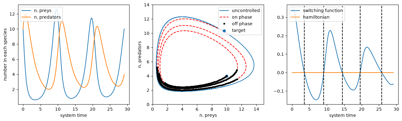
The time optimal trajectory is thus computed in the blink of an eye, showing us how to control the species dynamics in this example.