Jet transport in the simple pendulum

In this tutorial, which is inspired by an example in the documentation of the TaylorIntegration.jl package, we will be using the variational equations to propagate a small neighbourhood of initial conditions in the simple pendulum. This technique is called “jet transport” in the original example, in heyoka.py we call it evaluation of the Taylor map.

Let us begin with the formulation of the simple pendulum dynamics:

import heyoka as hy
dyn = hy.model.pendulum()

The pendulum() function generates the dynamics with respect to the state variables x (representing the angle with respect to the vertical) and v (which is the time derivative of x):

dyn

[(x, v), (v, -sin(x))]

We proceed then to the creation of a variational ODE system via the var_ode_sys class:

vsys = hy.var_ode_sys(dyn, hy.var_args.vars, order=8)

Here we asked for the variational equations up to order 8 with respect to the initial conditions of all state variables.

Next, we set up initial conditions for x and v:

# Initial conditions.
ic = [1.3, 0.0]

We are now ready to create a variational ODE integrator:

ta = hy.taylor_adaptive(vsys, ic, compact_mode=True)

We then proceed to define a small circular ring of displacements for the state variables x and v. This ring, which will be centered around the initial conditions ic, will represent the boundary of the neighbourhood in phase space that we will be propagating with the help of the variational equations:

import numpy as np
phi = np.linspace(0, 2*np.pi, 100)
r = 0.05

# Create the x and v displacements.
dxrng = r*np.cos(phi)
dvrng = r*np.sin(phi)

We can now proceed to the numerical integration of the variational ODE system. We will be integrating for a total of 6 libration periods of the pendulum, and we will be recording the state of the system (including the variational variables) 8 times per period:

# Compute the exact libration period of the pendulum
# via elliptic integrals.
from scipy.special import ellipk
T = 4*ellipk(np.sin(ic[0]/2)**2)

# Define a time grid over 6 periods, with
# 8 points per period.
tgrid = np.linspace(0, 6*T, 6*8+1)

# Run the numerical propagation.
res = ta.propagate_grid(tgrid)[-1]

We are now ready to compute and plot how the ring-shaped neighbourhood around the initial conditions ic evolves in time. In order to do so, we will be using the eval_taylor_map() method of the integrator class, as explained in the Taylor map computation tutorial:

%matplotlib inline

import matplotlib.pyplot as plt

fig = plt.figure(figsize=(6, 6))
ax = fig.gca()
ax.axis('equal')

colors = ['red', 'blue', 'green', 'purple',
          'orange', 'olive', 'gray', 'teal']

# Iterate over the states of the system
# computed at the grid points.
for j, cur_state in enumerate(res):
    # Assign the current state vector,
    # so that we can later invoke
    # ta.eval_taylor_map().
    ta.state[:] = cur_state

    # Compute the current state of the
    # ring-shaped neighbourhood.
    x_map = []
    v_map = []
    for i in range(0, len(dxrng)):
        tmp = ta.eval_taylor_map([dxrng[i], dvrng[i]])
        x_map.append(tmp[0])
        v_map.append(tmp[1])

    # Plot it.
    color=colors[j % len(colors)]
    plt.plot(x_map, v_map, zorder=-1, color=color, lw=.65)

    # Plot the propagated state as a
    # black dot.
    if j >= 8:
        continue
    circle = plt.Circle((ta.state[0], ta.state[1]),
                        0.015, color='k')
    ax.add_patch(circle)

plt.xlabel(r'$x$')
plt.ylabel(r'$v$');

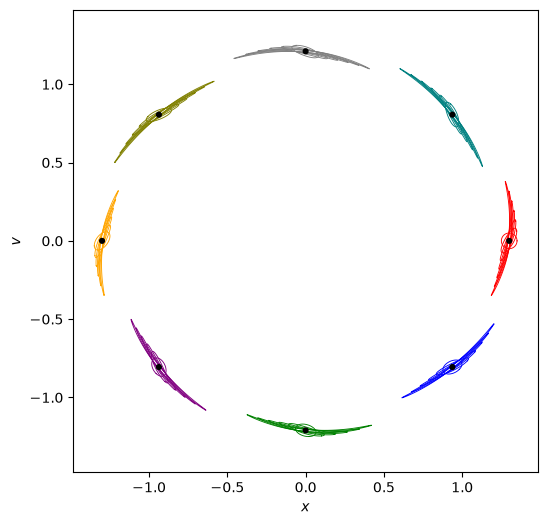
We can follow the evolution of the neighbourhood in phase space beginning with the red circular ring around the initial conditions [x=1.3, v=0]. As the state of the system (represented by black dots) circulates counterclockwise, we can see the ring progressively turning into an oval and stretching out.