Pseudo arc-length continuation in the CR3BP#
In this example we will refine the basic continuation scheme used in Continuation of Periodic Orbits in the CR3BP and use instead, as continuation parameter, the pseudo arc-length to obtain the family of Lyapunov orbits around L1.
The resulting numerical scheme allows to follow through folds of the curve implicitly defined by the periodicity condition and the Poincare’ phasing condition.
Preamble#
As usual, we make some standard imports:
import heyoka as hy
import numpy as np
import time

from scipy.optimize import least_squares, root_scalar
from copy import deepcopy

from matplotlib.pylab import plt

%matplotlib inline
… and define some functions that will help later on to visualize our trajectories and make nice plots. (ignore them and come back to this later in case you are curious)
def compute_L_points(mu, cf_px):
    """Computes The exact position of the Lagrangian points. To do so it finds the zeros of the
    the dynamics equation for px.

        Args:
            mu (float): The value of the mu parameter.
            cf_px (heyoka compiled function): The px dynamics equation. (will only depend on x,y,z,py)

        Returns:
            xL1, xL2, xL3, xL45, yL45: The coordinates of the various Lagrangian Points
    """
    # Position of the lagrangian points approximated
    xL1 = (mu - 1.0) + (mu / 3.0 / (1.0 - mu)) ** (1 / 3)
    xL2 = (mu - 1.0) - (mu / 3.0 / (1.0 - mu)) ** (1 / 3)
    xL3 = -(mu - 1.0) - 7.0 / 12.0 * mu / (1 - mu)
    yL45 = np.sin(60.0 / 180.0 * np.pi)
    xL45 = -0.5 + mu

    # Solve for the static equilibrium from the approximated solution (x,y,z,py)
    def equilibrium(expr, x, y):
        retval = cf_px([x, y, 0, x], pars=[mu])[0]
        return retval

    xL1 = root_scalar(lambda x: equilibrium(f, x, 0.0), x0=xL1, x1=xL1 - 1e-2).root
    xL2 = root_scalar(lambda x: equilibrium(f, x, 0.0), x0=xL2, x1=xL2 - 1e-2).root
    xL3 = root_scalar(lambda x: equilibrium(f, x, 0.0), x0=xL3, x1=xL3 - 1e-2).root
    return xL1, xL2, xL3, xL45, yL45


def potential_function(position, mu):
    """Computes the system potential
    Args:
        position (array-like): The position in Cartesian coordinates
        mu (float): The value of the mu parameter.

    Returns:
        The potential
    """
    x, y, z = position
    r_1 = np.sqrt((x - mu) ** 2 + y**2 + z**2)
    r_2 = np.sqrt((x - mu + 1) ** 2 + y**2 + z**2)
    Omega = 1.0 / 2.0 * (x**2 + y**2) + (1 - mu) / r_1 + mu / r_2
    return Omega


def jacobi_constant(state, mu):
    """Computes the system Jacobi constant
    Args:
        state (array-like): The system state (x,y,z,px,py,pz)
        mu (float): The value of the mu parameter.

    Returns:
        The Jacobi constant for the state
    """
    x, y, z, px, py, pz = state
    vx = px + y
    vy = py - x
    vz = pz
    r_1 = np.sqrt((x - mu) ** 2 + y**2 + z**2)
    r_2 = np.sqrt((x - mu + 1) ** 2 + y**2 + z**2)
    Omega = 1 / 2 * (x**2 + y**2) + (1 - mu) / r_1 + mu / r_2
    T = 1 / 2 * (vx**2 + vy**2 + vz**2)
    C = Omega - T
    return C
We now define the CR3BP equations … (see circular restricted three-body problem)
# Create the symbolic variables.
symbols_state = ["x", "y", "z", "px", "py", "pz"]
x = np.array(hy.make_vars(*symbols_state))
# This will contain the r.h.s. of the equations
f = []

rps_32 = ((x[0] - hy.par[0]) ** 2 + x[1] ** 2 + x[2] ** 2) ** (-3 / 2.0)
rpj_32 = ((x[0] - hy.par[0] + 1.0) ** 2 + x[1] ** 2 + x[2] ** 2) ** (-3 / 2.0)

# The r.h.s. of the equations of motion.
f.append(x[3] + x[1])
f.append(x[4] - x[0])
f.append(x[5])
f.append(
    x[4]
    - (1.0 - hy.par[0]) * rps_32 * (x[0] - hy.par[0])
    - hy.par[0] * rpj_32 * (x[0] - hy.par[0] + 1.0)
)
f.append(-x[3] - ((1.0 - hy.par[0]) * rps_32 + hy.par[0] * rpj_32) * x[1])
f.append(-((1.0 - hy.par[0]) * rps_32 + hy.par[0] * rpj_32) * x[2])
f = np.array(f)

# We compile the r.h.s. of the dynamics into compiled functions as to later be able to evaluate their numerical values magnitude.
cf_f = hy.cfunc(f, vars=x)
cf_px = hy.cfunc([f[3]], vars=[x[0], x[1], x[2], x[4]])  # x,y,z,py
and the corresponding variational equations (see and Continuation of Periodic Orbits in the CR3BP), which will be used to compute, in general, the state transition matrix \(\mathbf \Phi\).
symbols_phi = []
for i in range(6):
    for j in range(6):
        # Here we define the symbol for the variations
        symbols_phi.append("phi_" + str(i) + str(j))
phi = np.array(hy.make_vars(*symbols_phi)).reshape((6, 6))
dfdx = []
for i in range(6):
    for j in range(6):
        dfdx.append(hy.diff(f[i], x[j]))
dfdx = np.array(dfdx).reshape((6, 6))
# The (variational) equations of motion
dphidt = dfdx @ phi
Finally, we create the dynamics in the format requested by heyoka, including all 6 + 6x6 = 42 equations:
dyn = []
for state, rhs in zip(x, f):
    dyn.append((state, rhs))
for state, rhs in zip(phi.reshape((36,)), dphidt.reshape((36,))):
    dyn.append((state, rhs))
# These are the initial conditions on the variational equations (the identity matrix)
ic_var = np.eye(6).reshape((36,)).tolist()
and instantiate the Taylor integrator (high accuracy and no compact mode)
start_time = time.time()
ta = hy.taylor_adaptive(
    # The ODEs.
    dyn,
    # The initial conditions.
    [-0.45, 0.80, 0.00, -0.80, -0.45, 0.58] + ic_var,
    # Operate below machine precision
    # and in high-accuracy mode.
    tol=1e-18,
    high_accuracy=True,
)
print("--- %s seconds --- to build the Taylor integrator" % (time.time() - start_time))
--- 4.908559322357178 seconds --- to build the Taylor integrator
The Pseudo arc-length continuation method#
In the most general form, and in a nutshell, numerical continuation considers an equation in the form:
assumes a solution \(\underline{ \mathbf x}_0, \lambda_0\) is available and seeks a new solution \(\underline{ \mathbf x}_0+\delta\underline{\mathbf{x}}\) corrisponding to \(\lambda_0+\delta \lambda\). Pretty trivial right? Turns out its not. As \(\lambda\) varies, new solutions may appear, disappear bifurcate, fold, which makes it rather complicated!
In cases where the solution curve implicitly defined by \(\underline{{\mathbf G}}\) folds with respect to the continuation parameter \(\lambda\), we need to find a better parametrization. A common solution is to consider a new continuation parameter intrinsically linked to the solution curve geometry: the curve arc-length \(s\). Assuming as reference \(s=s_0\) in \(\underline{ \mathbf x}_0, \lambda_0\), the arc-length can be considered as a function of \(\underline{\mathbf{x}}\) and \(\lambda\). We can then write \(s = \tilde s\left(\underline{ \mathbf x}, \lambda\right)\).
Under this idea one can formally write:
or, equivalently:
where \(\underline{ \mathbf y} = [\underline{ \mathbf x}, \lambda ]\) and \(\underline{\mathbf G}^*=[\underline{\mathbf G}, \tilde s - s]\). Starting from the solution \([\underline{ \mathbf x}_0, \lambda_0], s_0\) we have reformulated the problem and may now seek a new solution \([\underline{ \mathbf x}_0+\delta\underline{\mathbf{x}}, \lambda_0+\delta \lambda]\) corresponding to \(s_0+\delta s\). We obtain (at least formally) a continuation scheme able to follow easily through folds of the \(\underline{ \mathbf x}, \lambda\) curve, since the \(\underline{ \mathbf y}, s\) curve has none! (the arc-length is always uniformly increasing along the solution curve).
The problem now is that we cannot really compute \(\tilde s\) easily! But we can approximate \(\delta s\) as the projection of \([\delta \underline{ \mathbf x}, \delta \lambda]\) onto the tangent vector \(\mathbf \tau = \left[\frac{d\underline{ \mathbf x}}{ds}, \frac{d\lambda}{ds}\right]\) (hence the name pseudo arc-length is used).
Eventually, the system:
is considered, and for a given increment of the pseudo arc-length \(\delta s\) is solved for \(\delta \underline{ \mathbf x}, \delta \lambda\).
The case of continuing periodic orbits.#
In the case of a search for periodic solutions to the system \(\dot{\underline{\mathbf x}} =\underline{ \mathbf f}(\underline{\mathbf x})\) we indicate the generic solution to this system as \(\underline{ \mathbf x}\left(t; \underline{ \mathbf x}_0\right)\) and may thus write the periodicity condition as:
We thus search for \(\underline{ \mathbf x}_0, T\) roots of the equation above. Assuming we have one such solution, we will slightly abuse the notation and omit a further \(0\) as a subscript in \(\underline{\mathbf x}_0\) indicating such an initial solution simply as as \(\underline{\mathbf x}_0, T_0\).
To continue this initial solution we seek \(\delta\underline{\mathbf x}\) and \(\delta T\) so that:
In other words we are perturbing our initial condition and period and demand to end up in a new periodic orbit. It is straight forward to see that for any fixed \(\delta T\) there is more than one \(\underline{ \mathbf x}_0\) that would do the trick. Infact any point on the whole new periodic orbit would work! Thus, as we saw also in Continuation of Periodic Orbits in the CR3BP, to recover a unique solution, we add the Poincare’ phasing condition and search, instead, for a solution to the system:
this system of seven equations is our \(\underline{{\mathbf G}} = \underline{\mathbf 0}\) with \(\delta T\) being our continuation parameter.
We now apply the pseudo arc-length condition to avoid issues when the solution curve folds for increasing periods.
We get:
which, with \(\delta s\) fixed, is an overdetermined system of 8 equations in the seven unknowns \(\delta\underline{\mathbf x}, \delta T\). Note also that \(\mathbf \tau\) is found differentiating with respect to the pseudo arc-length \(s\) our \(\underline{{\mathbf G}}\) considering both \(\delta\underline{\mathbf x}(s)\) and \(\delta T(s)\) as a function of \(s\) and then applying a normalization. We will solve the above system using a predictor corrector scheme.
Predictor#
If we expand in Taylor series the relation (2) we get:
which forms the basis to get a first guess (predictor) on the new continued state.
It is convenient to assemble the following matrix:
then, the predictor scheme, becomes:
# Single iteration from ic, t_final, ds
def predictor(x0, T0, ds):
    # 1 - We compute the state transition matrix Phi (integrating the full EOM for t_final)
    ta.time = 0.0
    ta.state[:] = x0.tolist() + ic_var
    out = ta.propagate_until(T0)
    Phi = ta.state[6:].reshape((6, 6))
    # 2 - We compute the dynamics f (at zero, but for periodic orbits this is the same at T)
    f_dyn = cf_f(x0, pars=[mu]).reshape(-1, 1)
    # 3 - Assemble the matrix A
    A = np.concatenate((Phi - np.eye(6), f_dyn.T))
    A = np.concatenate((A, np.insert(f_dyn, -1, 0).reshape((-1, 1))), axis=1)
    # 4 - Compute the tangent vector tau
    tauT = 1
    taux = -np.linalg.inv(A[:, :6].T @ A[:, :6]) @ (A[:, :6].T @ A[:, -1]) * tauT
    norm = np.sqrt(taux @ taux + tauT * tauT)
    tauT /= norm
    taux /= norm
    # 5 - Add to the matrix A
    tmp = np.insert(taux, 6, tauT).reshape(1, -1)
    A = np.concatenate((A, tmp))
    # 6 - Compute the b vector
    b = np.zeros((8, 1))
    b[7, 0] = ds
    # 6 - Predict an initial guess
    y = np.linalg.inv(A.T @ A) @ (A.T @ b)
    return y, taux, tauT
Lets instantiate our periodic solution. It is the same Lyapunov orbit we have used in the example Continuation of Periodic Orbits in the CR3BP.
# These conditions correspond to a Lyapunov orbit closeto the L2 point
ic = np.array(
    [
        -8.3660628427188066e-01,
        6.8716725011222035e-05,
        0.0000000000000000e00,
        -2.3615604665605682e-05,
        -8.3919863043620713e-01,
        0.0000000000000000e00,
    ]
)
t_final = 2.6915996001673941e00
mu = 0.01215057
ta.pars[0] = mu
# Pseudo arc-length
ds = 1e-3
# We call the predictor
predicted, taux, tauT = predictor(ic, t_final, ds)
Corrector#
We want to find \(\delta \underline{\mathbf y} = [\delta \underline{\mathbf{x}}, \delta T]\) so that the system of equations (2), reported again below for convenience, is satisfied: $\( (2) \qquad \left\{ \begin{array}{l} \underline{ \mathbf x}\left(T_0 + \delta T; \underline{ \mathbf x}_0 + \delta\underline{\mathbf x}\right) - \underline{ \mathbf x}_0 - \delta\underline{\mathbf x}= \mathbf 0 \\ \delta \underline{\mathbf x} \cdot \underline{\mathbf f} (\underline{ \mathbf x}_0) = 0 \\ \mathbf \tau \cdot [\delta \underline{ \mathbf x}, \delta T] = \delta s \end{array} \right. \)$ and can start from the guess returned by the predictor step.
Different methods can be used to solve the overdetermined system of equations above (which admits a unique solution), we here use the least-square method implemented in scipy and give our own implementation of a Newton based method.
First, we define a function that returns, for some \(\delta\underline{\mathbf y} = [\delta \underline{\mathbf{x}}, \delta T]\), the violations to the equations (2).
def full_system(X0, T0, dy, taux, tauT, ds):
    dx = deepcopy(dy[:6])
    dT = deepcopy(dy[6])
    x = X0 + dx
    propagation_time = T0 + dT
    # 1 - We compute the state at propagation_time
    ta.time = 0.0
    ta.state[:] = x.tolist() + ic_var
    out = ta.propagate_until(propagation_time)
    # 2 - We compute the dynamics f (at zero, but for periodic orbits this is the same at T)
    f_dyn0 = cf_f(X0, pars=[mu]).reshape(-1, 1)
    # 3 - Error on the state
    state_err = ta.state[:6] - x
    # Error on Poincare phasing
    poin_err = dx @ f_dyn0
    # Error on pseudo arc-length
    pseudo_err = taux @ dx + tauT * dT - ds
    # 4 - Assemble return value
    retval = np.insert(state_err, 6, poin_err)
    retval = np.insert(retval, 7, pseudo_err)
    Phi = ta.state[6:].reshape((6, 6))
    return retval, Phi
… we can then call the scipy.optimze.least_squares method to make such a violation vanish.
# A least squared corrector
def corrector_ls(X0, T0, dy0, taux, tauy, ds, tol=1e-12):
    sol = least_squares(
        lambda dy: full_system(X0, T0, dy, taux, tauT, ds)[0], dy0, ftol=tol
    )
    return sol.x
corrected_ls = corrector_ls(ic, t_final, predicted[:, 0], taux, tauT, ds, tol=1e-14)
We will inspect this result later. Now we implement our own Newton based method making use of the variational equations to compute the necessary gradient.
def corrector_Newton(
    X0, T0, dy, taux, tauy, ds, tol=1e-12, max_iter=100, verbose=False
):
    flag_tol = False

    curr_dx = deepcopy(dy[:6])
    curr_dT = deepcopy(dy[6])

    # Linearization point
    curr_x = X0 + curr_dx.T
    curr_T = T0 + curr_dT

    for i in range(max_iter):
        # 1 - We compute the state transition matrix Phi (integrating the full EOM from curr_x for t_final)
        ta.time = 0.0
        ta.state[:] = curr_x.tolist() + ic_var
        out = ta.propagate_until(curr_T)
        Phi = ta.state[6:].reshape((6, 6))
        # 2 - We compute the dynamics f (at the initial state)
        f_dyn0 = cf_f(X0, pars=[mu]).reshape(-1, 1)
        # 3 - We compute the dynamics f (at curr_T)
        f_dynT = cf_f(ta.state[:6], pars=[mu]).reshape(-1, 1)
        # 4 - Assemble the function (the full nonlinear system) value at the current point
        state_err = ta.state[:6] - curr_x
        # Error on Poincare phasing
        poin_err = curr_dx @ f_dyn0
        # Error on pseudo arc-length
        pseudo_err = taux @ curr_dx + tauT * curr_dT - ds
        b = np.zeros((8, 1))
        b[:6, 0] = -state_err
        b[6, 0] = -poin_err
        b[7, 0] = -pseudo_err
        if verbose:
            print(np.linalg.norm(state_err), poin_err, pseudo_err)
        toterror = (
            np.abs(np.linalg.norm(state_err)) + np.abs(poin_err) + np.abs(pseudo_err)
        )
        if toterror < tol:
            flag_tol = True
            break
        # 5 - Assemble the matrix A (gradient)
        A = np.concatenate((Phi - np.eye(6), f_dynT.T))
        A = np.concatenate((A, np.insert(f_dynT, -1, 0).reshape((-1, 1))), axis=1)
        # add the tau row
        tmp = np.insert(taux, 6, tauT).reshape(1, -1)
        A = np.concatenate((A, tmp))

        # Solve for new y = [dx, dT]
        y = (np.linalg.inv(A.T @ A) @ A.T @ b).reshape(
            -1,
        )
        curr_dx += y[:6]
        curr_dT += y[6]
        curr_x = X0 + curr_dx.T
        curr_T = T0 + curr_dT
    if verbose:
        if flag_tol:
            print("Exit condition - Accuracy")
        else:
            print("Exit condition - Maximum Iterations")
        print("Accuracy achieved: ", toterror)
        print("Iterations: ", i)
    return np.insert(curr_dx.T, 6, curr_dT)
corrected_N = corrector_Newton(
    ic, t_final, predicted[:, 0], taux, tauT, ds, tol=1e-14, verbose=False
)
We now assess if the system (2) is actually solved, and to what precision, in both cases:
errN = full_system(ic, t_final, corrected_N, taux, tauT, ds)[0]
err_ls = full_system(ic, t_final, corrected_ls, taux, tauT, ds)[0]
print("Error for the Newton method:", np.linalg.norm(errN))
print("Error for the Least-squares method:", np.linalg.norm(err_ls))
Error for the Newton method: 8.573824179843603e-15
Error for the Least-squares method: 1.2142886444425054e-12
And check the CPU time:
%timeit corrector_Newton(ic, t_final, predicted[:,0], taux, tauT, ds, tol=1e-14)
7.8 ms ± 24.2 µs per loop (mean ± std. dev. of 7 runs, 100 loops each)
%timeit corrector_ls(ic, t_final, predicted[:,0], taux, tauT, ds, tol=1e-14)
12.9 ms ± 63.2 µs per loop (mean ± std. dev. of 7 runs, 100 loops each)
Note that this CPU timing comparison is not entirely fair, as the least square solver is still integrating the variational equations, but not using the associated gradient information.
Producing the whole Lyapunov family#
We now use the code produced above to continue to a whole orbit family. We start defining an initial periodic orbit (around L1) and the starting point.
# These conditions correspond to a Lyapunov orbit close to the L1 point
ic = np.array(
    [
        -8.3660628427188066e-01,
        6.8716725011222035e-05,
        0.0000000000000000e00,
        -2.3615604665605682e-05,
        -8.3919863043620713e-01,
        0.0000000000000000e00,
    ]
)
period = 2.6915996001673941e00

# Starting point
new_ic = deepcopy(ic)
new_period = deepcopy(period)
# Pseudo arc-length increment
ds = 1e-3
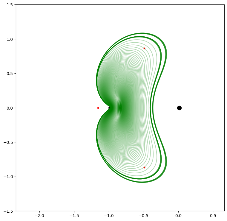
Finally we loop over the predictor-corrector and plot each orbit found.
plt.figure(figsize=(9, 9))

ax = plt.subplot(1, 1, 1)
# We find the postiion of the lagrangian points
xL1, xL2, xL3, xL45, yL45 = compute_L_points(mu, cf_px)

# Plot the lagrangian points and primaries
zoom = 1.5
ax.set_xlim(xL1 - zoom, xL1 + zoom)
ax.set_ylim(-zoom, +zoom)
ax.scatter(mu, 0, c="k", s=100)
ax.scatter(mu - 1, 0, c="k", s=30)
ax.scatter(xL1, 0, c="r", s=10)
ax.scatter(xL2, 0, c="r", s=10)
ax.scatter(xL3, 0, c="r", s=10)
ax.scatter(-0.5 + mu, yL45, c="r", s=10)
ax.scatter(-0.5 + mu, -yL45, c="r", s=10)

# Set to true to get more info on the iterations
verbose = True
start_time = time.time()
# Main iterations
for i in range(200):
    # We call the predictor
    predicted, taux, tauT = predictor(new_ic, new_period, ds)
    # We call the corrector, if it fails (A^tA goes singular) we decrease the pseudo arc-length and try again
    try:
        corrected_N = corrector_Newton(
            new_ic, new_period, predicted[:, 0], taux, tauT, ds, tol=1e-15
        )
        # Check convergence
        errN, Phi = full_system(new_ic, new_period, corrected_N, taux, tauT, ds)
        err = np.linalg.norm(errN)
        # Log
        if verbose:
            print("ds:", ds, "err:", err)
        # Accept the step
        if err < 1e-12:
            new_ic = new_ic + corrected_N[:6]
            new_period = new_period + corrected_N[6]
            if verbose:
                print("Converged - increase ds")
            ds *= 1.2
            if ds > 0.05:
                ds = 0.05
            # Reset the state
            ta.time = 0
            ta.state[:] = new_ic.tolist() + ic_var
            # Time grid
            t_grid = np.linspace(0, new_period, 2000)
            # Propagate
            out = ta.propagate_grid(t_grid)
            # Plot
            ax.plot(out[4][:, 0], out[4][:, 1], "g", alpha=0.3)
        # Reject the step
        else:
            ds /= 1.1
            if verbose:
                print("Low Precision - reducing ds")
    # The (A^T A) matrix was likely singular, we reduce the step ad try again.
    except:
        if verbose:
            print("Singular matrix - reducing ds")
        ds /= 1.1
print("--- %s seconds --- to do the iterations" % (time.time() - start_time))
ds: 0.001 err: 3.7125860080010274e-13
Converged - increase ds
ds: 0.0012 err: 1.1297503340463586e-13
Converged - increase ds
ds: 0.0014399999999999999 err: 2.0054823741788055e-13
Converged - increase ds
ds: 0.0017279999999999997 err: 7.624771600123291e-16
Converged - increase ds
ds: 0.0020735999999999997 err: 2.286492635797018e-13
Converged - increase ds
ds: 0.0024883199999999996 err: 3.167132102716876e-13
Converged - increase ds
ds: 0.0029859839999999993 err: 3.538672102411126e-14
Converged - increase ds
ds: 0.003583180799999999 err: 2.0052650646751112e-13
Converged - increase ds
ds: 0.0042998169599999985 err: 8.113302994273082e-13
Converged - increase ds
ds: 0.005159780351999998 err: 1.3803765177581485e-13
Converged - increase ds
Singular matrix - reducing ds
ds: 0.005628851293090906 err: 0.149162938277794
Low Precision - reducing ds
ds: 0.005117137539173551 err: 0.051661475165313685
Low Precision - reducing ds
Singular matrix - reducing ds
Singular matrix - reducing ds
ds: 0.0038445811714301653 err: 3.430258445004303e-16
Converged - increase ds
Singular matrix - reducing ds
ds: 0.004194088550651088 err: 0.18034373661749403
Low Precision - reducing ds
ds: 0.003812807773319171 err: 1.625453431156856e-13
Converged - increase ds
ds: 0.004575369327983005 err: 0.26047463481919153
Low Precision - reducing ds
ds: 0.0041594266618027315 err: 1.4697102368760275e-13
Converged - increase ds
ds: 0.004991311994163278 err: 0.015419299071966347
Low Precision - reducing ds
ds: 0.0045375563583302525 err: 0.009469637791999545
Low Precision - reducing ds
ds: 0.004125051234845684 err: 0.011685183396634347
Low Precision - reducing ds
ds: 0.0037500465771324394 err: 2.389957742578105e-13
Converged - increase ds
ds: 0.004500055892558927 err: 2.1565374580657768e-14
Converged - increase ds
Singular matrix - reducing ds
Singular matrix - reducing ds
Singular matrix - reducing ds
ds: 0.004057150316356658 err: 1.4423641477437126e-13
Converged - increase ds
Singular matrix - reducing ds
ds: 0.004425982163298171 err: 2.8616224763996445e-14
Converged - increase ds
Singular matrix - reducing ds
Singular matrix - reducing ds
ds: 0.004389403798312235 err: 1.3055592498534213e-13
Converged - increase ds
Singular matrix - reducing ds
ds: 0.004788440507249711 err: 3.217864177116722e-13
Converged - increase ds
ds: 0.005746128608699653 err: 0.06992557378073407
Low Precision - reducing ds
ds: 0.005223753280636048 err: 1.341698247013916e-13
Converged - increase ds
ds: 0.006268503936763257 err: 0.005025234270002906
Low Precision - reducing ds
ds: 0.005698639942512051 err: 6.332288055797163e-16
Converged - increase ds
Singular matrix - reducing ds
ds: 0.006216698119104055 err: 5.878029260535262e-14
Converged - increase ds
ds: 0.007460037742924866 err: 0.033000640636744266
Low Precision - reducing ds
Singular matrix - reducing ds
ds: 0.006165320448698235 err: 2.878597295091012e-13
Converged - increase ds
ds: 0.007398384538437882 err: 0.017468966290852112
Low Precision - reducing ds
ds: 0.006725804125852619 err: 2.264380956369148e-14
Converged - increase ds
ds: 0.008070964951023142 err: 0.1948631284448623
Low Precision - reducing ds
ds: 0.007337240864566492 err: 4.011561276684139e-13
Converged - increase ds
Singular matrix - reducing ds
ds: 0.008004262761345264 err: 1.4183758132511748e-14
Converged - increase ds
Singular matrix - reducing ds
ds: 0.008731923012376653 err: 7.59557369241061e-16
Converged - increase ds
ds: 0.010478307614851983 err: 0.12770158502714596
Low Precision - reducing ds
ds: 0.009525734195319983 err: 3.8761389911822585e-13
Converged - increase ds
Singular matrix - reducing ds
ds: 0.010391710031258163 err: 3.0922685544040364e-14
Converged - increase ds
ds: 0.012470052037509794 err: 3.7541886997112583
Low Precision - reducing ds
ds: 0.011336410943190722 err: 3.0173437599136796e-13
Converged - increase ds
ds: 0.013603693131828866 err: 1.8776040709339157
Low Precision - reducing ds
ds: 0.01236699375620806 err: 3.8396373049524095e-13
Converged - increase ds
ds: 0.01484039250744967 err: 9.872486436897804e-14
Converged - increase ds
Singular matrix - reducing ds
ds: 0.016189519099036 err: 2.7188488795189925e-13
Converged - increase ds
ds: 0.0194274229188432 err: 5.192799796231296
Low Precision - reducing ds
ds: 0.017661293562584723 err: 2.8653946061093254e-13
Converged - increase ds
ds: 0.021193552275101668 err: 3.8501413949480947e-13
Converged - increase ds
ds: 0.025432262730122 err: 2.58122186023138
Low Precision - reducing ds
ds: 0.023120238845565456 err: 3.4774246253792823e-13
Converged - increase ds
ds: 0.027744286614678548 err: 9.935463308476736e-17
Converged - increase ds
ds: 0.033293143937614254 err: 6.54354637446382e-14
Converged - increase ds
ds: 0.03995177272513711 err: 1.5783904342673787e-13
Converged - increase ds
ds: 0.047942127270164524 err: 1.1067649234811774e-13
Converged - increase ds
ds: 0.05 err: 1.3456491753155182e-13
Converged - increase ds
ds: 0.05 err: 7.482216503814388e-14
Converged - increase ds
ds: 0.05 err: 1.5246373543738397e-13
Converged - increase ds
ds: 0.05 err: 1.0078677159371306e-13
Converged - increase ds
ds: 0.05 err: 9.002415722394033e-14
Converged - increase ds
ds: 0.05 err: 1.0296838851901742e-13
Converged - increase ds
ds: 0.05 err: 4.1455700820911174e-14
Converged - increase ds
ds: 0.05 err: 7.131803764333485e-16
Converged - increase ds
ds: 0.05 err: 1.8063250990405207e-14
Converged - increase ds
ds: 0.05 err: 3.3908410377789977e-16
Converged - increase ds
ds: 0.05 err: 3.441818122443283e-14
Converged - increase ds
ds: 0.05 err: 8.7957153495834295e-16
Converged - increase ds
ds: 0.05 err: 1.1372989150881946e-14
Converged - increase ds
ds: 0.05 err: 9.690607920382238e-14
Converged - increase ds
ds: 0.05 err: 1.8635452571530917e-14
Converged - increase ds
ds: 0.05 err: 7.983055637968554e-16
Converged - increase ds
ds: 0.05 err: 5.993212895406073e-16
Converged - increase ds
ds: 0.05 err: 2.0289838488322305e-14
Converged - increase ds
ds: 0.05 err: 6.154788100814035e-14
Converged - increase ds
ds: 0.05 err: 7.651699203854313e-16
Converged - increase ds
ds: 0.05 err: 1.2026369088486011e-14
Converged - increase ds
ds: 0.05 err: 1.511607119500301e-14
Converged - increase ds
ds: 0.05 err: 4.912962735469023e-14
Converged - increase ds
ds: 0.05 err: 6.343537887303993e-14
Converged - increase ds
ds: 0.05 err: 4.7818799763473866e-15
Converged - increase ds
ds: 0.05 err: 1.9407209421085858e-14
Converged - increase ds
ds: 0.05 err: 2.5341312390563286e-14
Converged - increase ds
ds: 0.05 err: 1.7300060983268164e-15
Converged - increase ds
ds: 0.05 err: 2.8117467340799274e-13
Converged - increase ds
ds: 0.05 err: 1.3362058579616174e-14
Converged - increase ds
ds: 0.05 err: 9.973485199941996e-14
Converged - increase ds
ds: 0.05 err: 1.1873892552131126e-14
Converged - increase ds
ds: 0.05 err: 3.4229547630308305e-15
Converged - increase ds
ds: 0.05 err: 1.907785506068812e-14
Converged - increase ds
ds: 0.05 err: 4.511912919782471e-14
Converged - increase ds
ds: 0.05 err: 9.716432218626694e-14
Converged - increase ds
ds: 0.05 err: 8.493977248872996e-14
Converged - increase ds
ds: 0.05 err: 8.62310704665012e-14
Converged - increase ds
ds: 0.05 err: 5.4596566744817414e-14
Converged - increase ds
ds: 0.05 err: 7.477709144723294e-14
Converged - increase ds
ds: 0.05 err: 2.7164244925118436e-14
Converged - increase ds
ds: 0.05 err: 1.9280921131629667e-14
Converged - increase ds
ds: 0.05 err: 9.75261896974471e-14
Converged - increase ds
ds: 0.05 err: 1.1499456264153612e-13
Converged - increase ds
ds: 0.05 err: 1.9448481389021904e-13
Converged - increase ds
ds: 0.05 err: 1.8830927479301792e-14
Converged - increase ds
ds: 0.05 err: 8.008435717638159e-14
Converged - increase ds
ds: 0.05 err: 1.8875664171478675e-13
Converged - increase ds
ds: 0.05 err: 4.455272104008286e-15
Converged - increase ds
ds: 0.05 err: 4.101955144813206e-14
Converged - increase ds
ds: 0.05 err: 8.404081058855128e-14
Converged - increase ds
ds: 0.05 err: 6.472469550979843e-14
Converged - increase ds
ds: 0.05 err: 1.4897465385710178e-13
Converged - increase ds
ds: 0.05 err: 1.3923778634122624e-13
Converged - increase ds
ds: 0.05 err: 1.4950457681466991e-13
Converged - increase ds
ds: 0.05 err: 7.409535573221516e-14
Converged - increase ds
ds: 0.05 err: 2.8689867040676603e-13
Converged - increase ds
ds: 0.05 err: 1.2585163165342884e-13
Converged - increase ds
ds: 0.05 err: 6.944488666827651e-14
Converged - increase ds
ds: 0.05 err: 9.54256918559437e-14
Converged - increase ds
ds: 0.05 err: 6.459553023071906e-14
Converged - increase ds
ds: 0.05 err: 5.469116515527568e-16
Converged - increase ds
ds: 0.05 err: 1.0245913069182179e-13
Converged - increase ds
ds: 0.05 err: 7.872008135451232e-14
Converged - increase ds
ds: 0.05 err: 9.452915082956397e-14
Converged - increase ds
ds: 0.05 err: 1.9728161024691671e-13
Converged - increase ds
ds: 0.05 err: 8.352474066684535e-14
Converged - increase ds
ds: 0.05 err: 2.607727729570358e-13
Converged - increase ds
ds: 0.05 err: 4.4030867985545686e-13
Converged - increase ds
ds: 0.05 err: 4.178680978230548e-13
Converged - increase ds
ds: 0.05 err: 3.6150333345673875e-14
Converged - increase ds
ds: 0.05 err: 2.052899938371835e-14
Converged - increase ds
ds: 0.05 err: 2.1709237863474563e-13
Converged - increase ds
ds: 0.05 err: 2.481517083313343e-14
Converged - increase ds
ds: 0.05 err: 1.6667483873960702e-13
Converged - increase ds
ds: 0.05 err: 1.1114200227112883e-13
Converged - increase ds
ds: 0.05 err: 5.971506893507456e-13
Converged - increase ds
ds: 0.05 err: 5.236929657476717e-13
Converged - increase ds
ds: 0.05 err: 4.647676965288109e-13
Converged - increase ds
ds: 0.05 err: 6.528573726768541e-13
Converged - increase ds
ds: 0.05 err: 1.6576011362708567e-13
Converged - increase ds
ds: 0.05 err: 4.8127052021903455e-14
Converged - increase ds
ds: 0.05 err: 3.340066738158382e-13
Converged - increase ds
ds: 0.05 err: 6.115455647526132e-13
Converged - increase ds
ds: 0.05 err: 5.032120381970581e-13
Converged - increase ds
ds: 0.05 err: 7.346060551629237e-14
Converged - increase ds
ds: 0.05 err: 5.673060172729317e-13
Converged - increase ds
ds: 0.05 err: 5.557741647428475e-13
Converged - increase ds
ds: 0.05 err: 5.342250092207268e-13
Converged - increase ds
ds: 0.05 err: 5.068997424180067e-13
Converged - increase ds
ds: 0.05 err: 6.958147505875287e-13
Converged - increase ds
ds: 0.05 err: 4.1661702213243113e-13
Converged - increase ds
ds: 0.05 err: 1.2895814498241862e-12
Low Precision - reducing ds
ds: 0.045454545454545456 err: 4.203304666732572e-13
Converged - increase ds
ds: 0.05 err: 8.378936949409995e-13
Converged - increase ds
ds: 0.05 err: 6.855876211857165e-13
Converged - increase ds
ds: 0.05 err: 1.1857427677765994e-13
Converged - increase ds
ds: 0.05 err: 3.2132042846197704e-14
Converged - increase ds
ds: 0.05 err: 1.3840157305490845e-12
Low Precision - reducing ds
ds: 0.045454545454545456 err: 2.1616922930711222e-13
Converged - increase ds
ds: 0.05 err: 4.3779000957518755e-13
Converged - increase ds
ds: 0.05 err: 7.445362225587346e-13
Converged - increase ds
ds: 0.05 err: 2.2212170886710085e-13
Converged - increase ds
ds: 0.05 err: 2.759765655699936e-13
Converged - increase ds
ds: 0.05 err: 2.991591717944264e-13
Converged - increase ds
ds: 0.05 err: 4.240699098193959e-13
Converged - increase ds
ds: 0.05 err: 1.4867726209365809e-12
Low Precision - reducing ds
ds: 0.045454545454545456 err: 3.714710009910772e-13
Converged - increase ds
ds: 0.05 err: 3.320001895982378e-13
Converged - increase ds
ds: 0.05 err: 1.3345255229097643e-12
Low Precision - reducing ds
ds: 0.045454545454545456 err: 5.763617913996049e-13
Converged - increase ds
ds: 0.05 err: 7.622530488848844e-14
Converged - increase ds
ds: 0.05 err: 2.945182791978049e-13
Converged - increase ds
ds: 0.05 err: 3.46917543178887e-13
Converged - increase ds
ds: 0.05 err: 7.13173005572568e-14
Converged - increase ds
ds: 0.05 err: 1.3494830722439872e-13
Converged - increase ds
ds: 0.05 err: 3.707524212441393e-13
Converged - increase ds
ds: 0.05 err: 1.0957701123735237e-12
Low Precision - reducing ds
ds: 0.045454545454545456 err: 6.598927257681549e-13
Converged - increase ds
ds: 0.05 err: 5.502167330033484e-13
Converged - increase ds
ds: 0.05 err: 1.1037243528416048e-13
Converged - increase ds
ds: 0.05 err: 5.366584929284795e-13
Converged - increase ds
ds: 0.05 err: 1.6327601978892026e-12
Low Precision - reducing ds
ds: 0.045454545454545456 err: 2.2077920524903307e-13
Converged - increase ds
ds: 0.05 err: 6.699297467780139e-13
Converged - increase ds
ds: 0.05 err: 1.8792988984636516e-13
Converged - increase ds
--- 35.786818504333496 seconds --- to do the iterations