Poincaré sections

In this example, we will be using heyoka.py’s event detection feature to compute a Poincaré section for a particular case of the Arnold-Beltrami-Childress (ABC) flow. The system of ODEs reads:

\[\begin{split} \begin{cases} \dot{x} = \sin z + \frac{3}{4} \cos y\\ \dot{y} = \sin x + \cos z\\ \dot{z} = \frac{3}{4} \sin y + \cos x \end{cases}, \end{split}\]

and we will consider the intersection of the flow with the plane defined by \(y = 0\).

We begin as usual with the definition of the symbolic state variables \(x\), \(y\) and \(z\):

import heyoka as hy
x, y, z = hy.make_vars("x", "y", "z")

Next, we create the ODE system:

sys = [(x, 3/4.*hy.cos(y) + hy.sin(z)),
       (y, hy.cos(z) + hy.sin(x)),
       (z, hy.cos(x) + 3/4.*hy.sin(y))]

In order to detect when the solution crosses the \(y=0\) plane, we will be using a non-terminal event. The event’s callback will compute and store in a list the value of the \(x\) and \(z\) coordinates when the solution crosses the \(y=0\) plane.

# The list of (x, z) values when the solution
# crosses the y = 0 plane.
xz_list = []

# The event's callback.
def cb(ta, t, d_sgn):
    # Compute the state of the system
    # at the event trigger time.
    ta.update_d_output(t)

    # Add the (x, z) coordinates to xz_list.
    xz_list.append((ta.d_output[0], ta.d_output[2]))

# Create the non-terminal event.
ev = hy.nt_event(
    # The lhs of the event equation.
    y,
    # The callback.
    cb)

We can now proceed to create the integrator. We set the initial conditions to \(x=y=z=0\) (to be changed later) and we pass to the constructor the non-terminal event that we just created:

ta = hy.taylor_adaptive(sys, [0., 0., 0.], nt_events = [ev])

We will now generate a grid of initial conditions in \(\left[0, 2\pi \right]\) for \(x\) and \(z\), and, for each set of initial conditions, we will integrate the system up to \(t=1000\). At the end of each integration, we will append to map_list the list of \(\left( x, z \right)\) coordinates at which the trajectory intersected the \(y=0\) plane:

import numpy as np

map_list = []

# Grid of 13 x 13 initial conditions.
for xg in np.linspace(0, 2*np.pi, 13):
    for zg in np.linspace(0, 2*np.pi, 13):
        # Reset time and initial conditions
        # in the integrator.
        ta.time = 0
        ta.state[:] = [xg, 0, zg]
        
        # Clear up xz_list.
        xz_list.clear()
        
        # Integrate up to t=1000.
        ta.propagate_until(1000.)
        
        # Reduce the values of x and z modulo 2*pi.
        xz_arr = np.mod(np.array(xz_list), np.pi*2)
        
        # Add the intersection points to map_list,
        # if there's enough of them.
        if xz_arr.shape[0] > 50:
            map_list.append(xz_arr)

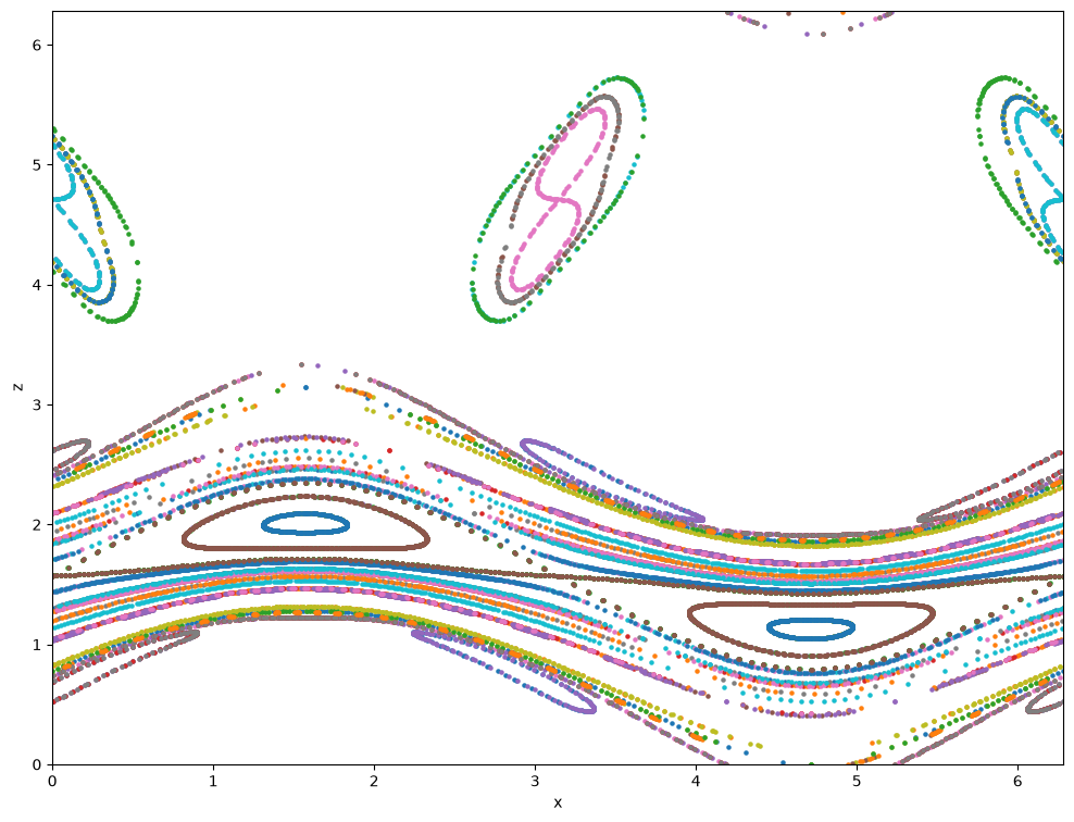
We can now plot the Poincaré section:

from matplotlib.pylab import plt

fig = plt.figure(figsize=(12, 9))
for m in map_list:
    plt.scatter(m[:, 0], m[:, 1], s=5)
plt.xlim((0,2*np.pi))
plt.ylim((0,2*np.pi))
plt.xlabel('x')
plt.ylabel('z');