Feed-Forward Neural Networks

In this tutorial, we will introduce feed-forward neural networks (FFNNs) in heyoka.py, and how to use heyoka.py FFNN factory to create FFNNs. For an example on how to load a FFNN model from torch to heyoka.py, please check out: Interfacing torch to heyoka.py; while for an example on applications of FFNNs in dynamical systems, check out: Neural Hamiltonian ODE and Neural ODEs.

To facilitate the instantiation of FFNNs, heyoka.py implements, in its module model, a Feed Forward Neural Network factory called ffnn(). The Neural Network inputs \(\mathbf {in}\), with dimensionality \(n_{in}\) are fed into a succession of \(N \ge 0 \) neural layers defined by:

\[ \mathbf h_i = F_i(\mathbf W_i\mathbf h_{i-1} + \mathbf b_i), \quad i = 1 .. N \]

to derive the Neural Network outputs \(\mathbf {out}\) with dimensionality \(n_{out}\):

\[ \mathbf {out} = F_{N+1}(\mathbf W_{N+1}\mathbf h_{N} + \mathbf b_{N+1}) \]

where \(\mathbf h_0 = \mathbf {in}\) and \(F_i\) define the network non-linearities, or activation functions.

We here show how to use this factory in the context of inference as well as in definition of the dynamics of an adaptive Taylor integrator. We start with importing the tools we need:

import heyoka as hy
import numpy as np

%matplotlib inline
import matplotlib.pyplot as plt

Let us start with something simple and small, without hidden layers and with one only input and output, to illustrate the basics of such a factory.

# We create the symbols for the network inputs (only one in this first simple case)
x = hy.make_vars("x")

# We define as nonlinearity a simple linear layer
linear = lambda inp: inp

# We call the factory to construct the FFNN:
ffnn = hy.model.ffnn(inputs = [x], nn_hidden = [], n_out = 1, activations = [linear])
print(ffnn)

[((p0 * x) + p1)]

The factory ffnn() returns a list of heyoka.expression representing each of the output neurons, in this case only one. The same syntax can be used to instantiate a more complex case:

x, y = hy.make_vars("x", "y")
ffnn = hy.model.ffnn(inputs = [x, y], nn_hidden = [32], n_out = 2, activations = [hy.tanh, linear])
print(ffnn)

[((p64 * tanh(((p0 * x) + (p1 * y) + p128))) + (p65 * tanh(((p2 * x) + (p3 * y) + p129))) + (p66 * tanh(((p4 * x) + (p5 * y) + p130))) + (p67 * tanh(((p6 * x) + (p7 * y) + p131))) + (p68 * tanh(((p8 * x) + (p9 * y) + p132))) + (p69 * tanh(((p10 * x) + (p11 * y) + p133))) + (p70 * tanh(((p12 * x) + (p13 * y) + p134))) + (p71 * tanh(((p14 * x) + (p15 * y) + p135))) + (p72 * tanh(((p16 * x) + (p17 * y) + p136))) + (p73 * tanh(((p18 * x) + (p19 * y) + p137))) + (p74 * tanh(((p20 * x) + (p21 * y) + p138))) + (p75 * tanh(((p22 * x) + (p23 * y) + p139))) + (p76 * tanh(((p24 * x) + (p25 * y) + p140))) + (p77 * tanh(((p26 * x) + (p27 * y) + p141))) + (p78 * tanh(((p28 * x) + (p29 * y) + p142))) + (p79 * tanh(((p30 * x) + (p31 * y) + p143))) + (p80 * tanh(((p32 * x) + (p33 * y) + p144))) + (p81 * tanh(((p34 * x) + (p35 * y) + p145))) + (p82 * tanh(((p36 * x) + (p37 * y) + p146))) + (p83 * tanh(((p38 * x) + (p39 * y) + p147))) + (p84 * tanh(((p40 * x) + (p41 * y) + p148))) + (p85 * tanh(((p42 * x) + ..., ((p96 * tanh(((p0 * x) + (p1 * y) + p128))) + (p97 * tanh(((p2 * x) + (p3 * y) + p129))) + (p98 * tanh(((p4 * x) + (p5 * y) + p130))) + (p99 * tanh(((p6 * x) + (p7 * y) + p131))) + (p100 * tanh(((p8 * x) + (p9 * y) + p132))) + (p101 * tanh(((p10 * x) + (p11 * y) + p133))) + (p102 * tanh(((p12 * x) + (p13 * y) + p134))) + (p103 * tanh(((p14 * x) + (p15 * y) + p135))) + (p104 * tanh(((p16 * x) + (p17 * y) + p136))) + (p105 * tanh(((p18 * x) + (p19 * y) + p137))) + (p106 * tanh(((p20 * x) + (p21 * y) + p138))) + (p107 * tanh(((p22 * x) + (p23 * y) + p139))) + (p108 * tanh(((p24 * x) + (p25 * y) + p140))) + (p109 * tanh(((p26 * x) + (p27 * y) + p141))) + (p110 * tanh(((p28 * x) + (p29 * y) + p142))) + (p111 * tanh(((p30 * x) + (p31 * y) + p143))) + (p112 * tanh(((p32 * x) + (p33 * y) + p144))) + (p113 * tanh(((p34 * x) + (p35 * y) + p145))) + (p114 * tanh(((p36 * x) + (p37 * y) + p146))) + (p115 * tanh(((p38 * x) + (p39 * y) + p147))) + (p116 * tanh(((p40 * x) + (p41 * y) + p148))) + (p117 * ...]

The resulting screen output of the built expression is much longer and eventually it actually makes little sense to print it.

Note

The user must take care of consistency of the dimensions of the various kwargs passed into the factory, else an error will be raised. For example, the dimension of the list containing the activation functions must be exactly one more than the dimension of the nn_hidden and so on.

All the network parameters, i.e. the weights and biases, are, by default, defined as par[j] in the heyoka expression system. This flattens the weight matrices \(\mathbf W_i, i=1 .. (N-1)\) and then the biases \(\mathbf b_i, i=1 .. (N-1)\) into one non-dimensional vector. In this case we have that \(\mathbf W_1\) is a (2,32) matrix, \(\mathbf W_2\) is a (32,2) matrix, \(\mathbf b_1\) is a (32,1) vector and \(\mathbf b_2\) a (2,1) vector. A total of 2x32+32x2+32+2=162 parameters are then needed.

We now assume the matrices and biases are available (for example from some third party code that trained the model) and for the sake of the tutorial we create them here randomly. In case you are familiar with the ML tool pytorch, check the dedicated example Interfacing torch to heyoka.py.

# To simulate that the network parameters are coming from some third party tool that performed the network training, 
# we here generate them as random numpy arrays.
W1 = 0.5 - np.random.random((2,32))
W2 = 0.5 - np.random.random((32,2))
b1 =  0.5 - np.random.random((32,1))
b2 =  0.5 - np.random.random((2,1))

And we flatten them into the heyoka format (i.e. first weights then biases):

flattened_nw = np.concatenate((W1.flatten(), W2.flatten(), b1.flatten(), b2.flatten()))

Inference

In order to use the ffnn to make inferences, we must compile it into a cfunction. Thats easy though, specially if you have followed the compiled functions tutorial:

cf = hy.cfunc(ffnn, [x, y])
print(cf)

C++ datatype: double
Variables: [x, y]
Output #0: ((p64 * tanh(((p0 * x) + (p1 * y) + p128))) + (p65 * tanh(((p2 * x) + (p3 * y) + p129))) + (p66 * tanh(((p4 * x) + (p5 * y) + p130))) + (p67 * tanh(((p6 * x) + (p7 * y) + p131))) + (p68 * tanh(((p8 * x) + (p9 * y) + p132))) + (p69 * tanh(((p10 * x) + (p11 * y) + p133))) + (p70 * tanh(((p12 * x) + (p13 * y) + p134))) + (p71 * tanh(((p14 * x) + (p15 * y) + p135))) + (p72 * tanh(((p16 * x) + (p17 * y) + p136))) + (p73 * tanh(((p18 * x) + (p19 * y) + p137))) + (p74 * tanh(((p20 * x) + (p21 * y) + p138))) + (p75 * tanh(((p22 * x) + (p23 * y) + p139))) + (p76 * tanh(((p24 * x) + (p25 * y) + p140))) + (p77 * tanh(((p26 * x) + (p27 * y) + p141))) + (p78 * tanh(((p28 * x) + (p29 * y) + p142))) + (p79 * tanh(((p30 * x) + (p31 * y) + p143))) + (p80 * tanh(((p32 * x) + (p33 * y) + p144))) + (p81 * tanh(((p34 * x) + (p35 * y) + p145))) + (p82 * tanh(((p36 * x) + (p37 * y) + p146))) + (p83 * tanh(((p38 * x) + (p39 * y) + p147))) + (p84 * tanh(((p40 * x) + (p41 * y) + p148))) + (p85 * tanh(((p42 * x) + ...
Output #1: ((p96 * tanh(((p0 * x) + (p1 * y) + p128))) + (p97 * tanh(((p2 * x) + (p3 * y) + p129))) + (p98 * tanh(((p4 * x) + (p5 * y) + p130))) + (p99 * tanh(((p6 * x) + (p7 * y) + p131))) + (p100 * tanh(((p8 * x) + (p9 * y) + p132))) + (p101 * tanh(((p10 * x) + (p11 * y) + p133))) + (p102 * tanh(((p12 * x) + (p13 * y) + p134))) + (p103 * tanh(((p14 * x) + (p15 * y) + p135))) + (p104 * tanh(((p16 * x) + (p17 * y) + p136))) + (p105 * tanh(((p18 * x) + (p19 * y) + p137))) + (p106 * tanh(((p20 * x) + (p21 * y) + p138))) + (p107 * tanh(((p22 * x) + (p23 * y) + p139))) + (p108 * tanh(((p24 * x) + (p25 * y) + p140))) + (p109 * tanh(((p26 * x) + (p27 * y) + p141))) + (p110 * tanh(((p28 * x) + (p29 * y) + p142))) + (p111 * tanh(((p30 * x) + (p31 * y) + p143))) + (p112 * tanh(((p32 * x) + (p33 * y) + p144))) + (p113 * tanh(((p34 * x) + (p35 * y) + p145))) + (p114 * tanh(((p36 * x) + (p37 * y) + p146))) + (p115 * tanh(((p38 * x) + (p39 * y) + p147))) + (p116 * tanh(((p40 * x) + (p41 * y) + p148))) + (p117 * ...

Let us now make an inference of the input point [1.2, -2.2]

cf([1.2,-2.2], pars = flattened_nw)

array([ 1.49511131, -0.80492322])

The drawback here is that at each inference the actual values of all the parameters must be copied into the expression upon evaluation, which may result in slower performances. Hardcoding the values into the FFNN is surely a better option, which can be achieved using the optional kwarg nn_wb (neural network weights and biases) of the factory ffnn():

ffnn = hy.model.ffnn(inputs = [x, y], nn_hidden = [32], n_out = 2, activations = [hy.tanh, linear], nn_wb = flattened_nw)
print(ffnn)

[(0.22338470042538006 + (0.21547147783988052 * tanh((-0.26675552677982872 - (0.48394040738268840 * x) - (0.28249692952967353 * y)))) + (0.48976066454601108 * tanh(((0.40739175638945957 * x) - 0.0012203733632745184 - (0.37540969828850446 * y)))) + (0.38601192275129104 * tanh((-0.43059183238980159 - (0.31877694134335366 * x) - (0.48864687912249438 * y)))) + (0.43823445509804160 * tanh(((0.46362115016063166 * x) - 0.085051785553607040 - (0.26484738387068285 * y)))) + (0.39528716573695888 * tanh((0.12486390940366110 + (0.10580443938420381 * x) - (0.32244759504897658 * y)))) + (0.20252491662566663 * tanh((0.017407675178997217 + (0.19563578486242506 * x) - (0.48029175427673232 * y)))) + (0.14596835209534065 * tanh(((0.45038139278996092 * x) + (0.35325222259336631 * y) - 0.11253391948151525))) + (0.46796001700943912 * tanh((0.48032540432491422 + (0.42074832398380246 * x) - (0.34591440923951422 * y)))) + (0.051690310127470163 * tanh(((0.10050842800052429 * x) + (0.45588998563494865 * y) - 0.15141897022543038))) + ..., ((0.41304314692150135 * tanh(((0.46362115016063166 * x) - 0.085051785553607040 - (0.26484738387068285 * y)))) + (0.12145864597261880 * tanh((0.12486390940366110 + (0.10580443938420381 * x) - (0.32244759504897658 * y)))) + (0.39843131562878664 * tanh(((0.45038139278996092 * x) + (0.35325222259336631 * y) - 0.11253391948151525))) + (0.044071316555207907 * tanh((0.024622445533577175 + (0.25747510475675850 * x) + (0.34497415704189516 * y)))) + (0.46788422838514609 * tanh((0.48032540432491422 + (0.42074832398380246 * x) - (0.34591440923951422 * y)))) + (0.40453807103855666 * tanh(((0.10050842800052429 * x) + (0.45588998563494865 * y) - 0.15141897022543038))) + (0.21613491820475716 * tanh(((0.15719015398740122 * x) + (0.084282103858048352 * y) - 0.23508217973906609))) + (0.38104401514976949 * tanh(((0.26660641785456951 * x) + (0.25579652211696524 * y) - 0.44755295414243501))) + (0.013288709701727908 * tanh((-0.094923330487312607 - (0.074043355987776671 * x) - (0.19218465281494101 * y)))) + (0.46172192520909927 * ...]

We can now recompile the function:

cf = hy.cfunc(ffnn, [x, y])
print(cf)

C++ datatype: double
Variables: [x, y]
Output #0: (0.22338470042538006 + (0.21547147783988052 * tanh((-0.26675552677982872 - (0.48394040738268840 * x) - (0.28249692952967353 * y)))) + (0.48976066454601108 * tanh(((0.40739175638945957 * x) - 0.0012203733632745184 - (0.37540969828850446 * y)))) + (0.38601192275129104 * tanh((-0.43059183238980159 - (0.31877694134335366 * x) - (0.48864687912249438 * y)))) + (0.43823445509804160 * tanh(((0.46362115016063166 * x) - 0.085051785553607040 - (0.26484738387068285 * y)))) + (0.39528716573695888 * tanh((0.12486390940366110 + (0.10580443938420381 * x) - (0.32244759504897658 * y)))) + (0.20252491662566663 * tanh((0.017407675178997217 + (0.19563578486242506 * x) - (0.48029175427673232 * y)))) + (0.14596835209534065 * tanh(((0.45038139278996092 * x) + (0.35325222259336631 * y) - 0.11253391948151525))) + (0.46796001700943912 * tanh((0.48032540432491422 + (0.42074832398380246 * x) - (0.34591440923951422 * y)))) + (0.051690310127470163 * tanh(((0.10050842800052429 * x) + (0.45588998563494865 * y) - 0.15141897022543038))) + ...
Output #1: ((0.41304314692150135 * tanh(((0.46362115016063166 * x) - 0.085051785553607040 - (0.26484738387068285 * y)))) + (0.12145864597261880 * tanh((0.12486390940366110 + (0.10580443938420381 * x) - (0.32244759504897658 * y)))) + (0.39843131562878664 * tanh(((0.45038139278996092 * x) + (0.35325222259336631 * y) - 0.11253391948151525))) + (0.044071316555207907 * tanh((0.024622445533577175 + (0.25747510475675850 * x) + (0.34497415704189516 * y)))) + (0.46788422838514609 * tanh((0.48032540432491422 + (0.42074832398380246 * x) - (0.34591440923951422 * y)))) + (0.40453807103855666 * tanh(((0.10050842800052429 * x) + (0.45588998563494865 * y) - 0.15141897022543038))) + (0.21613491820475716 * tanh(((0.15719015398740122 * x) + (0.084282103858048352 * y) - 0.23508217973906609))) + (0.38104401514976949 * tanh(((0.26660641785456951 * x) + (0.25579652211696524 * y) - 0.44755295414243501))) + (0.013288709701727908 * tanh((-0.094923330487312607 - (0.074043355987776671 * x) - (0.19218465281494101 * y)))) + (0.46172192520909927 * ...

And compute the inference much more efficiently as:

cf([1.2,-2.2])

array([ 1.49511131, -0.80492322])

Using the batch evaluation results in even faster code:

cf([[1.2,-2.2,1.0],[-2.2, -0.1,0.1]]).transpose()

array([[ 1.49511131, -0.80492322],
       [-0.82343905, -1.4238613 ],
       [ 0.2543584 , -0.04793984]])

Use in numerical integration

In a number of cases the right hand side of a system of ordinary differential equations contain an artificial neural network (ANN). This is the case, for example, in controlled systems where the state-feedback is provided via a neural network, or in those cases where the ANN has been trained to describe nonlinear interactions or external disturbances, but also in more advanced scenarios where the full system of ODEs is a ANN trained to reproduce some observed or desired dynamics. It is the case, as we shall see later, where a perturtbation to the system Hamiltonian is parametrized by an ANN, hence the name of this tutorial!

Note

A particularly significant case, in the context of Taylor integration, is also when the ANN is used to represent some otherwise discontinuous or non differentiable term, allowing the use of a Taylor integration also in those, otherwise untractable, cases.

Regardless of the reason why, we end up solving a system in the form:

\[ \dot {\mathbf x} = \mathbf f(\mathbf x, \mathcal N_\theta(\mathbf x)) \]

where we have denoted with \(\theta\) the network model parameters.

Making inferences of ANN in heyoka can surely be useful for debugging and other purposes, but it is likely not the main reason we use heyoka in the first place, nor the main objective of this tutorial. Instantiating and integrating a system in the form:

\[ \dot {\mathbf x} = \mathbf f(\mathbf x, \mathcal N_\theta(\mathbf x)) \]

is!

Let us then define a simple harmonic oscillator, perturbed by a random nonlinear term defined via an Artificial Neural Network:

\[\begin{split} \begin{array}{l} \dot x = v_x \\ \dot y = v_y \\ \dot v_x = - k_x x + \alpha \mathcal N_x \\ \dot v_y = - k_y y + \alpha \mathcal N_y \\ \end{array} \end{split}\]

Let us start defining the neural network.

x, y, vx, vy = hy.make_vars("x","y","vx","vy")

# Network parameters (play around)
nn_hidden = [10, 10]
activations = [hy.tanh, hy.tanh, hy.tanh] # the output will be in [-1,1]
n_inputs = 4
n_outputs = 2
nn_layers = [n_inputs] + nn_hidden + [n_outputs]

# Weight matrices
Ws = []
for i in range(0, len(activations)):
    Ws.append(0.5 - np.random.random((nn_layers[i], nn_layers[i+1])))
# Bias vectors
bs = []
for i in range(0, len(activations)):
    bs.append(np.random.random((nn_layers[i+1],1)))
# Flatten everything
flattened_nw =  np.concatenate([it.flatten() for it in Ws] + [it.flatten() for it in bs])

# Calling the ffnn factory
ffnn = hy.model.ffnn(inputs = [x, y, vx, vy], nn_hidden = nn_hidden, n_out = 2, activations = activations, nn_wb = flattened_nw)

We write the dynamics, introducing as heyoka parameters \(k_x, k_y\) and the value \(\alpha\) which will determine the strength of the perturbation.

x, y, vx, vy = hy.make_vars("x", "y", "vx", "vy")
dxdt = vx
dydt = vy
dvxdt = -hy.par[0] * x + hy.par[2] * ffnn[0]
dvydt = -hy.par[1] * y + hy.par[2] * ffnn[1]

and package it into a taylor_adaptive integrator which will compile the Taylor integrator for us and create the object we will use to perform numerics:

ta = hy.taylor_adaptive(
    # The ODEs.
    [(x, dxdt), (y, dydt), 
     (vx, dvxdt), (vy, dvydt)],
    # The initial conditions.
    [0., 1., 1., 0.],
    tol = 1e-16,
    compact_mode = True
)

We may now call the integrator. Let us start with the unperturbed case:

ta.state[:] = [0., 1., 1., 0.]
ta.time = 0
ta.pars[:] = [1,1,0.0]
tgrid = np.linspace(0,40,1000)
sol = ta.propagate_grid(tgrid)

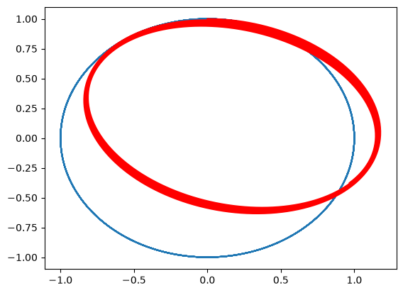
… to then assume the FFNN is perturbing the dynamics with some relatively small strength.

ta.state[:] = [0., 1., 1., 0.]
ta.time = 0
ta.pars[:] = [1,1,0.2]
tgrid = np.linspace(0,40,1000)
sol_pert = ta.propagate_grid(tgrid)

plt.plot(sol[5][:,0], sol[5][:,1])
plt.plot(sol_pert[5][:,0], sol_pert[5][:,1], 'r')

[<matplotlib.lines.Line2D at 0x7f47a7a9e230>]

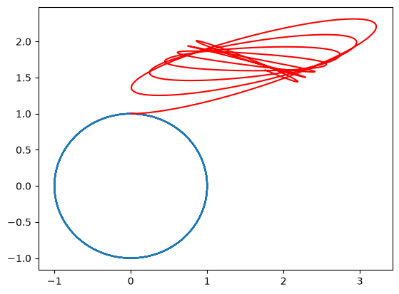
… increasing the perturbation level:

ta.state[:] = [0., 1., 1., 0.]
ta.time = 0
ta.pars[:] = [1,1,2.]
tgrid = np.linspace(0,40,1000)
sol_pert_strong = ta.propagate_grid(tgrid)

plt.plot(sol[5][:,0], sol[5][:,1])
plt.plot(sol_pert_strong[5][:,0], sol_pert_strong[5][:,1], 'r')

[<matplotlib.lines.Line2D at 0x7f47a67b47f0>]

… and thats all I wanted to tell you! But wait …. one last thing … the above system is dissipative and does not really look Hamiltonian right? The random perturbation is, well …. random. To fix this, have a look at the tutorial: Neural Hamiltonian ODE.