Ensemble propagations

Starting with version 0.17.0, heyoka.py offers support for ensemble propagations. In ensemble mode, multiple distinct instances of the same ODE system are integrated in parallel, typically using different sets of initial conditions and/or runtime parameters. Monte Carlo simulations and parameter searches are two typical examples of tasks in which ensemble mode is particularly useful.

The ensemble mode API mirrors the time-limited propagation functions available in the adaptive integrator class. Specifically, three functions are available:

• ensemble_propagate_until(), for ensemble propagations up to a specified epoch,

• ensemble_propagate_for(), for ensemble propagations for a time interval,

• ensemble_propagate_grid(), for ensemble propagations over a time grid.

In this tutorial, we will be focusing on the ensemble_propagate_until() function, but adapting the code to the other two functions should be straightforward.

At this time, ensemble propagations can use multiple threads of executions or multiple processes to achieve parallelisation. In the future, additional parallelisation modes (e.g., distributed) may be added.

A simple example

As usual, for this illustrative tutorial we will be using the ODEs of the simple pendulum. Thus, let us begin with the definition of the symbolic variables and of an integrator object:

import heyoka as hy

x, v = hy.make_vars("x", "v")

# Create the integrator object.
ta = hy.taylor_adaptive(
                        # Definition of the ODE system:
                        # x' = v
                        # v' = -9.8 * sin(x)
                        sys = [(x, v),
                         (v, -9.8 * hy.sin(x))],
                        # Initial conditions for x and v.
                        state = [0. ,0.])

Note how, differently from the other tutorials, here we have set the initial conditions to zeroes. This is because, in ensemble mode, we will never use directly the ta object to perform a numerical integration. Rather, ta acts as a template from which other integrator objects will be constructed, and thus its initial conditions are inconsequential.

The ensemble_propagate_until() function takes in input at least 4 arguments:

• the template integrator ta,

• the final epoch t for the propagations (this argument would be a time interval delta_t for ensemble_propagate_for() and a time grid for ensemble_propagate_grid()),

• the number of iterations n_iter in the ensemble,

• a function object gen, known as the generator.

The generator is a callable that takes two input arguments:

• a deep copy of the template integrator ta, and

• an iteration index idx in the [0, n_iter) range.

gen is then expected to modify the copy of ta (e.g., by setting its initial conditions to specific values) and return it.

The ensemble_propagate_until() function iterates over the [0, n_iter) range. At each iteration, the generator gen is invoked, with the template integrator as the first argument and the current iteration number as the second argument. The propagate_until() member function is then called on the integrator returned by gen, and the result of the propagation is appended to a list of results which is finally returned by ensemble_propagate_until() once all the propagations have finished.

Let us see a concrete example of ensemble_propagate_until() in action. First, we begin by creating 10 sets of different initial conditions to be used in the ensemble propagations:

# Create 10 sets of random initial conditions,
# one for each element of the ensemble.
import numpy as np

ensemble_ics = np.array([0.05, 0.025]) + np.random.uniform(-1e-2, 1e-2, (10, 2))

Next, we define a generator that will pick a set of initial conditions from ensemble_ics, depending on the iteration index:

# The generator.
def gen(ta_copy, idx):
    # Reset the time to zero.
    ta.time = 0.
    
    # Fetch initial conditions from ensemble_ics.
    ta_copy.state[:] = ensemble_ics[idx]

    return ta_copy

We are now ready to invoke the ensemble_propagate_until() function:

# Run the ensemble propagation up to t = 20.
ret = hy.ensemble_propagate_until(ta, 20., 10, gen)

The value returned by ensemble_propagate_until() is a list of tuples constructed by concatenating the integrator object used for each integration and the tuple returned by each propagate_until() invocation. This way, at the end of an ensemble propagation it is possible to inspect both the state of each integrator object and the output of each invocation of propagate_until() (including, e.g., the continuous output, if requested).

For instance, let us take a look at the first value in ret:

ret[0]

(C++ datatype            : double
 Tolerance               : 2.220446049250313e-16
 High accuracy           : false
 Compact mode            : false
 Taylor order            : 20
 Dimension               : 2
 Time                    : 20
 State                   : [0.052242519580864545, 0.06328528188764432],
 <taylor_outcome.time_limit: -4294967299>,
 0.19786971536716183,
 0.22041086857062708,
 98,
 None,
 None)

The first element of the tuple is the integrator object that was used in the invocation of propagate_until(). The remaining elements of the tuple are the output of the propagate_until() invocation (i.e., integration outcome, min/max timestep, etc., as detailed in the adatpive integrator tutorial).

The ensemble_propagate_until() function can be invoked with additional optional keyword arguments, beside the mandatory initial 4:

• the algorithm keyword argument is a string that specifies the parallelisation algorithm that will be used by ensemble_propagate_until(). The supported values are currently "thread" (the default) and "process" (see below for a discussion of the pros and cons of each method);

• the max_workers keyword argument is an integer that specifies how many workers are spawned during parallelisation. Defaults to None, see the Python docs for a detailed explanation;

• the chunksize keyword argument is an integer that specifies the size of the tasks that are submitted to the parallel workers. Defaults to 1, see the Python docs for a detailed explanation. This keyword argument applies only to the process parallelisation method.

Any other keyword argument passed to ensemble_propagate_until() will be forwarded to the propagate_until() invocations.

Let us see a comprehensive example with multiple keyword arguments:

ret = hy.ensemble_propagate_until(ta, 20., 10, gen,
                                  # Use no more than 8 worker threads.
                                  max_workers = 8,
                                  # Request continuous output.
                                  c_output = True
                                 )

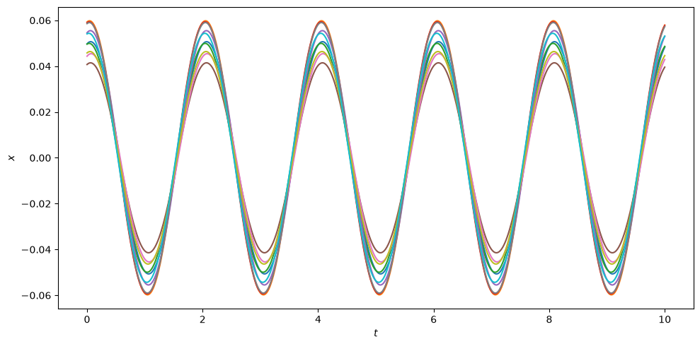
Let us now use the continuous output to plot the evolution of the \(x\) coordinate over time for each element of the ensemble:

from matplotlib.pylab import plt

fig = plt.figure(figsize=(10, 5))

# Create a time range.
t_rng = np.linspace(0, 10., 500)

for tup in ret:
    # Fetch the continuous output function object.
    c_out = tup[5]

    plt.plot(t_rng, c_out(t_rng)[:,0])

plt.xlabel("$t$")
plt.ylabel("$x$")
plt.tight_layout();

Choosing between threads and processes

Ensemble propagations default to using multiple threads of execution for parallelisation. Multithreading usually performs better than multiprocessing, however there are at least two big caveats to keep in mind when using multithreading:

• first, it is the user’s responsibility to ensure that the user-provided function objects such as the generator and the callbacks (if present) are safe for use in a multithreaded context. In particular, the following actions will be performed concurrently by separate threads of execution:

  • invocation of the generator’s call operator. That is, the generator is shared among several threads of execution and used concurrently;

  • deep copy of the events callbacks and invocation of the call operator on the copies. That is, each thread of execution gets its own copy of the event callbacks thanks to the creation of a new integrator object via the generator;

  • concurrent execution of copies of the step callback, if present. That is, before multithreaded execution starts, n_iter deep copies of the step callback (if present) are made, with each iteration in the ensemble propagation using its own exclusive copy of the step callback.

  For instance, an event callback which performs write operations on a global variable without using some form of synchronisation will result in unpredictable behaviour when used in an ensemble propagation.

• second, due to the global interpreter lock (GIL), Python is typically not able to execute code concurrently from multiple threads. Thus, if a considerable portion of the integration time if spent executing user-defined callbacks, ensemble simulations will exhibit poor parallel speedup.

As an alternative, it is possible to use multiple processes (instead of threads) when performing ensemble propagations by passing the keyword argument algorithm="process". Processes have a higher initial creation overhead, but they also feature two important advantages:

• there are no safety concerns regarding data sharing, as each process gets its own copy of all the data necessary to perform an integration;

• the GIL performance issues are avoided because there are multiple Python interpreters running in parallel (rather than multiple threads sharing exclusive access to a single interpreter), and thus ensemble propagations with event detection may parallelise more efficiently when using multiprocessing.

When employing multiprocessing, users should be aware that the chunksize keyword argument can have a big influence on performance. Please see the explanation in the Python docs for more detailed information.