ODEs with parameters

The values of numerical constants in heyoka.py can either be specified when constructing an ODE system, or they can be loaded at a later stage when the ODE system is being integrated. The latter type of numerical constant is known as a parameter.

Let’s start by importing heyoka.py and NumPy:

import heyoka as hy
import numpy as np

For this example, we will be integrating the pendulum ODE:

\[\begin{split} \begin{cases} x^\prime = v \\ v^\prime = -g \sin x \end{cases}, \end{split}\]

where \(g\) is the value of the gravitational acceleration (\(9.8\,\mathrm{m}/\mathrm{s}^2\) on Earth). Let’s first create the symbolic state variables \(x\) and \(v\), which represent respectively the pendulum’s angle and its time derivative:

x, v = hy.make_vars("x", "v")

Because we don’t want to fix \(g\) to a specific numerical value, when writing down the ODE system we will be implementing \(g\) as a parameter:

ode_sys = [(x, v),
           (v, -hy.par[0] * hy.sin(x))]

The syntax par[0] means that the actual value of \(g\) will be the first value (index 0) loaded from the parameter array when integrating the ODE system.

Let’s now create the integrator object, using as initial conditions \(\left( \pi/2, 0\right)\):

ta = hy.taylor_adaptive(ode_sys,
                       [np.pi/2, 0.])

print(ta)

C++ datatype            : double
Tolerance               : 2.220446049250313e-16
High accuracy           : false
Compact mode            : false
Taylor order            : 20
Dimension               : 2
Time                    : 0
State                   : [1.5707963267948966, 0]
Parameters              : [0]

As you can see from the screen output Parameters = ..., heyoka.py detected that ode_sys contains one parameter, and set its value to zero. We can change the value of the parameter by directly accessing the parameters array:

ta.pars[0] = 9.8

print(ta)

C++ datatype            : double
Tolerance               : 2.220446049250313e-16
High accuracy           : false
Compact mode            : false
Taylor order            : 20
Dimension               : 2
Time                    : 0
State                   : [1.5707963267948966, 0]
Parameters              : [9.8]

Note that it is also possible to directly set the value of the parameters on construction via the pars keyword argument:

ta = hy.taylor_adaptive(ode_sys,
                       [np.pi/2, 0.],
                       pars=[9.8])

print(ta)

C++ datatype            : double
Tolerance               : 2.220446049250313e-16
High accuracy           : false
Compact mode            : false
Taylor order            : 20
Dimension               : 2
Time                    : 0
State                   : [1.5707963267948966, 0]
Parameters              : [9.8]

Let’s now integrate the ODE system for a few time units:

t_grid = np.linspace(0,10,1000)
e_hist = ta.propagate_grid(t_grid)[5][:,0]

Let’s now move to Mars, where the gravitational acceleration on the surface is \(3.71\,\mathrm{m}/\mathrm{s}^2\) (instead of good ole Earth’s \(9.8\,\mathrm{m}/\mathrm{s}^2\)):

# Reset time and state.
ta.time = 0
ta.state[:] = [np.pi/2, 0]

# Change gravity.
ta.pars[0] = 3.71

# Integrate again.
m_hist = ta.propagate_grid(t_grid)[5][:,0]

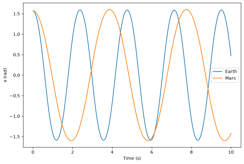
Finally, let’s plot the evolution of \(x\) in time to show how a pendulum swings more slowly on Mars:

from matplotlib.pylab import plt

fig = plt.figure(figsize=(9,6))

plt.plot(t_grid, e_hist, label="Earth")
plt.plot(t_grid, m_hist, label="Mars")
plt.xlabel("Time (s)")
plt.ylabel("x (rad)")
plt.legend();