
Note
Starting with heyoka.py 4.0.0, the tidal model introduced in this tutorial can be formulated more easily and more efficiently with the builtin support for Lagrangian and Hamiltonian mechanics. Nevertheless, this tutorial is kept in its original form as an example of advanced interoperability with SymPy.
Elastic tides#
In this tutorial, we will be formulating a simple 2D toy model of tidal interactions between a planet and its moon. The moon will be represented as a simple point mass, whereas the planet will be represented by a semi-rigid system of point masses which can be deformed by the tidal force. Although this is just a toy model, it will nevertheless be able to reproduce qualitatively some aspects of the complex spin-orbits interactions between a planet and its moon.
This example will also give us a chance to exercise more thoroughly the interoperability between heyoka.py and SymPy. In particular, we will be using SymPy’s classical mechanics module to formulate the equations of motion, which we will then proceed to numerically integrate with heyoka.py.
What to expect?#
Tides raised by a point-like moon create a distortion (more precisely, a bulge) in the distribution of matter in an otherwise spherical planet, which alters over time both the orbit of the moon and the rotational state of the planet. If the rotational angular velocity of the planet is greater (resp., smaller) than the orbital angular velocity of the moon, the moon’s orbit moves outward (resp., inward) and the rotational angular velocity of the planet decreases (resp., increases).
For instance: in the Earth-Moon system, the Earth’s rotation’s period (24 hours) is smaller than the Moon’s orbital period (28 days), and, as a consequence, the Moon slowly migrates outwards while Earth’s rotation slows down.
Vice-versa, the orbital period of Mars’ moon Phobos is shorter than a Martian day, and, as a consequence, the orbit of Phobos shrinks by about \(2\,\mathrm{cm}/y\) while Mars’ rotational velocity increases (albeit by a very small amount).
Our toy model should be able to reproduce both these scenarios.
Spokes on the wheel#
Let us begin by introducing the planet’s physical model. It consists of a central point mass \(m_0\) from which \(N\) massless rigid spokes of length \(a\) radiate at regular intervals. A spring is attached at the end of each spoke, and a small point mass \(m_i\) is attached to each spring. The masses \(m_i\) are constrained to move onto the spokes, and the springs are at rest when the masses \(m_i\) are at the end of the spokes. Here’s a picture for \(N=8\):
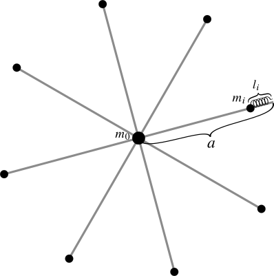
\(l_i\) represents the distance of \(m_i\) from the end of its spoke, with the convention that \(a - l_i\) is the distance of \(m_i\) from \(m_0\). When \(l_i\) becomes negative, \(m_i\) moves away from the end of the spoke while remaining always constrained to the spoke’s direction (i.e., as if the spoke extended to infinity).
The first Lagrangian#
As a first step, we begin by formulating the Lagrangian of the system without the moon. The generalised coordinates for this system can be chosen as
where \(\left(x_0, y_0\right)\) are the Cartesian coordinates of \(m_0\), \(l_i\), as explained above, is the distance of \(m_i\) from the end of its spoke, and \(\alpha\) is a rotation angle encoding the orientation of the wheel. Without loss of generality, we choose \(\alpha\) as the angle between the direction of the inertial \(x\) axis and the the direction of the spoke of the first mass \(m_1\). The Cartesian coordinates of \(m_i\) are then:
We can now formulate the kinetic energy for this system:
Without gravity, the only potential in the system is the elastic energy due to the springs:
where \(k\) is a spring constant assumed to be the same for all springs.
We can now begin to write the Lagrangian with SymPy. We start off by defining a few constants:
# Number of spokes.
N = 8
# Gravitational constant
# (will be used later).
G = 1.0
# Central mass m_0 and smaller masses m_i.
m0 = 10.0
masses = [0.05] * N
# Length of the spokes (i.e., rest position
# of the springs).
a = 1.0
We then introduce the spring constant \(k\) as a symbolic variable, so that we can change it later without recomputing everything. We will call it "par[0]" so that, when converting the SymPy expressions to heyoka.py, \(k\) will be interpreted as the runtime parameter at index 0:
from sympy import Symbol
k = Symbol("par[0]")
Next, we define the dynamical variables as prescribed by SymPy’s classical mechanics module:
from sympy.physics.mechanics import dynamicsymbols as ds, LagrangesMethod
# Generalised coordinates.
x0, y0, alpha = ds("x0 y0 alpha")
ljs = [ds("l{}".format(_ + 1)) for _ in range(N)]
# Generalised velocities (i.e., first-order
# time derivatives of the coordinates).
vx0, vy0, valpha = ds("x0 y0 alpha", 1)
vljs = [ds("l{}".format(_ + 1), 1) for _ in range(N)]
We will also need the definitions of \(x_i\) and \(y_i\) in order to formulate the kinetic energy term:
import sympy
xjs = [x0 + (a - ljs[_]) * sympy.cos(alpha + _ * (2 / N * sympy.pi)) for _ in range(N)]
yjs = [y0 + (a - ljs[_]) * sympy.sin(alpha + _ * (2 / N * sympy.pi)) for _ in range(N)]
We are now ready to formulate the kinetic energy:
T = 1 / 2.0 * m0 * (vx0**2 + vy0**2) + 1 / 2.0 * sum(
[masses[_] * (xjs[_].diff("t") ** 2 + yjs[_].diff("t") ** 2) for _ in range(N)]
)
Note how we used SymPy’s differentiation capabilities to compute the time derivatives of \(x_i\) and \(y_i\). Next is the potential energy term:
V = 1 / 2.0 * k * sum([ljs[_] ** 2 for _ in range(N)])
And the Lagrangian:
L = T - V
The symbolic expression of the Lagrangian is already looking quite complicated:
print(L)
-0.5*par[0]*(l1(t)**2 + l2(t)**2 + l3(t)**2 + l4(t)**2 + l5(t)**2 + l6(t)**2 + l7(t)**2 + l8(t)**2) + 0.025*(-(1.0 - l1(t))*sin(alpha(t))*Derivative(alpha(t), t) - cos(alpha(t))*Derivative(l1(t), t) + Derivative(x0(t), t))**2 + 0.025*((1.0 - l1(t))*cos(alpha(t))*Derivative(alpha(t), t) - sin(alpha(t))*Derivative(l1(t), t) + Derivative(y0(t), t))**2 + 0.025*(-(1.0 - l2(t))*sin(alpha(t) + 0.25*pi)*Derivative(alpha(t), t) - cos(alpha(t) + 0.25*pi)*Derivative(l2(t), t) + Derivative(x0(t), t))**2 + 0.025*((1.0 - l2(t))*cos(alpha(t) + 0.25*pi)*Derivative(alpha(t), t) - sin(alpha(t) + 0.25*pi)*Derivative(l2(t), t) + Derivative(y0(t), t))**2 + 0.025*(-(1.0 - l3(t))*sin(alpha(t) + 0.5*pi)*Derivative(alpha(t), t) - cos(alpha(t) + 0.5*pi)*Derivative(l3(t), t) + Derivative(x0(t), t))**2 + 0.025*((1.0 - l3(t))*cos(alpha(t) + 0.5*pi)*Derivative(alpha(t), t) - sin(alpha(t) + 0.5*pi)*Derivative(l3(t), t) + Derivative(y0(t), t))**2 + 0.025*(-(1.0 - l4(t))*sin(alpha(t) + 0.75*pi)*Derivative(alpha(t), t) - cos(alpha(t) + 0.75*pi)*Derivative(l4(t), t) + Derivative(x0(t), t))**2 + 0.025*((1.0 - l4(t))*cos(alpha(t) + 0.75*pi)*Derivative(alpha(t), t) - sin(alpha(t) + 0.75*pi)*Derivative(l4(t), t) + Derivative(y0(t), t))**2 + 0.025*(-(1.0 - l5(t))*sin(alpha(t) + 1.0*pi)*Derivative(alpha(t), t) - cos(alpha(t) + 1.0*pi)*Derivative(l5(t), t) + Derivative(x0(t), t))**2 + 0.025*((1.0 - l5(t))*cos(alpha(t) + 1.0*pi)*Derivative(alpha(t), t) - sin(alpha(t) + 1.0*pi)*Derivative(l5(t), t) + Derivative(y0(t), t))**2 + 0.025*(-(1.0 - l6(t))*sin(alpha(t) + 1.25*pi)*Derivative(alpha(t), t) - cos(alpha(t) + 1.25*pi)*Derivative(l6(t), t) + Derivative(x0(t), t))**2 + 0.025*((1.0 - l6(t))*cos(alpha(t) + 1.25*pi)*Derivative(alpha(t), t) - sin(alpha(t) + 1.25*pi)*Derivative(l6(t), t) + Derivative(y0(t), t))**2 + 0.025*(-(1.0 - l7(t))*sin(alpha(t) + 1.5*pi)*Derivative(alpha(t), t) - cos(alpha(t) + 1.5*pi)*Derivative(l7(t), t) + Derivative(x0(t), t))**2 + 0.025*((1.0 - l7(t))*cos(alpha(t) + 1.5*pi)*Derivative(alpha(t), t) - sin(alpha(t) + 1.5*pi)*Derivative(l7(t), t) + Derivative(y0(t), t))**2 + 0.025*(-(1.0 - l8(t))*sin(alpha(t) + 1.75*pi)*Derivative(alpha(t), t) - cos(alpha(t) + 1.75*pi)*Derivative(l8(t), t) + Derivative(x0(t), t))**2 + 0.025*((1.0 - l8(t))*cos(alpha(t) + 1.75*pi)*Derivative(alpha(t), t) - sin(alpha(t) + 1.75*pi)*Derivative(l8(t), t) + Derivative(y0(t), t))**2 + 5.0*Derivative(x0(t), t)**2 + 5.0*Derivative(y0(t), t)**2
We are now ready to form the Euler-Lagrange equations. First we need to construct a LagrangesMethod instance passing in the Lagrangian and the list of generalised coordinates:
LM = LagrangesMethod(L, [x0, y0, alpha] + ljs)
Next, we ask for the formulation of the equations:
LM.form_lagranges_equations();
The Euler-Lagrange equations are constructed by SymPy in a way which is not directly suitable for numerical integration (unless a solver for ODEs in implicit form is being used). In order to render the equations explicit, a system of symbolic linear equations needs to be solved. This can be done by invoking the rhs() method:
# Construct the Euler-Lagrange equations
# in explicit form.
LM_rhs = LM.rhs()
Warning
Do NOT try to print these equations to screen! The reason for this warning will be apparent in a moment.
We are now almost ready to convert the equations from SymPy to heyoka.py, but, before doing so, there is an issue that needs to be addressed. The equations contain the coordinates and their time derivatives as undefined functions of time, which heyoka.py’s elementary expression system does not understand. We will thus define a substitution dictionary that we will then use to replace the coordinates and velocities with plain variables while converting the equations to heyoka.py:
import heyoka as hy
# Create the substitution dictionary,
# mapping the SymPy coordinates and velocities
# to heyoka.py variables.
subs_dict = {
x0: hy.expression("x0"),
y0: hy.expression("y0"),
alpha: hy.expression("alpha"),
vx0: hy.expression("vx0"),
vy0: hy.expression("vy0"),
valpha: hy.expression("valpha"),
}
subs_dict = {
**subs_dict,
**dict((ljs[_], hy.expression("l{}".format(_ + 1))) for _ in range(N)),
**dict((vljs[_], hy.expression("vl{}".format(_ + 1))) for _ in range(N)),
}
We can now proceed to convert the symbolic equations of motion to heyoka.py:
# Convert LM_rhs to heyoka.py.
rhs_hy = map(lambda _: hy.from_sympy(_, subs_dict), LM_rhs)
# Generate the ODE system in the heyoka.py format.
eqs_hy = list(
zip(
[
hy.expression(_)
for _ in ["x0", "y0", "alpha"]
+ list("l{}".format(_ + 1) for _ in range(N))
+ ["vx0", "vy0", "valpha"]
+ list("vl{}".format(_ + 1) for _ in range(N))
],
rhs_hy,
)
)
Let us take a look at the size of the symbolic expressions in the ODE system (here measured as the number of nodes in the expression tree):
# Calculate the length of the rhs
# of each equation.
[len(_[1]) for _ in eqs_hy]
[1,
1,
1,
1,
1,
1,
1,
1,
1,
1,
1,
11525717900,
11525717900,
5762861487,
2881434641,
1440731719,
720413467,
360364035,
180691423,
91932239,
50557499,
36731043]
The first half of the ODE system is trivial, as expected. The size of the second half, however, is gigantic. How did this happen and why didn’t the computer crash?
The expressions exploded in size when SymPy had to solve a system of symbolic equations in order to bring the Euler-Lagrange equations in explicit form. The end result is a set of very large expressions which however feature a high degree of internal repetition. Thanks to the use of reference semantics, multiple “copies” of the same subexpression do not require additional storage, and thus SymPy is able to represent these large expressions without exhausting the system’s memory. Starting from version 0.15, heyoka.py also adopts reference semantics in the representation of expressions, and it is thus also able to cope with large expressions with frequent internal repetitions.
We can now proceed to the creation of the heyoka.py integrator object:
ta = hy.taylor_adaptive(eqs_hy, [0.0] * (6 + N * 2), compact_mode=True)
The length of the Taylor decomposition confirms indeed that the large expressions were simplified drastically during the construction of the integrator:
len(ta.decomposition)
1683
We are now ready to take our wobbly planet out for a spin. First we set a specific value for the spring constant:
# The spring constant is the runtime
# parameter at index 0.
ta.pars[0] = 5.0
Then we generate random initial velocities:
import numpy as np
# Reset time and state (useful for re-runs
# of this cell).
ta.time = 0
ta.state[:] = 0
# Generate random velocities.
ta.state[3 + N :] = (np.random.rand(3 + N) * 2 - 1) / 2.0
We can now proceed to the numerical integration:
time_grid = np.linspace(0, 20, 1000)
out = ta.propagate_grid(time_grid)
Before plotting a pretty animation, we precompute some quantities useful for visualisation purposes:
# Time evolution of m0.
r0_hist = out[-1][:, 0:2]
# Time evolution of the rotation angle.
alpha_hist = out[-1][:, 2]
# Time evolution of the smaller masses.
l_hist = [out[-1][:, 3 + _] for _ in range(N)]
r_hist = [
r0_hist
+ np.array(
[
(a - l_hist[_]) * np.cos(alpha_hist + _ * (2.0 / N * np.pi)),
(a - l_hist[_]) * np.sin(alpha_hist + _ * (2.0 / N * np.pi)),
]
).transpose()
for _ in range(N)
]
# Compute the time evolution of the barycentre
# of the system.
bar_hist = np.sum(
np.array([_[0] * _[1] for _ in zip([m0] + masses, [r0_hist] + r_hist)]), axis=0
) / np.sum([m0] + masses)
And here comes the animation:
%%capture
import matplotlib.pyplot as plt
from matplotlib import animation, rc
from IPython.display import HTML
from scipy import interpolate
fig = plt.figure(figsize=(8, 8))
ax = plt.subplot(111)
# Init the graphical elements.
tc0 = plt.Circle((0.2, 0.0), 0.03, ec="black", fc="black", zorder=3)
tcs = [plt.Circle((0.2, 0.0), 0.01, ec="black", fc="black", zorder=3) for _ in range(N)]
tc_bar = plt.Circle((0.2, 0.0), 0.01, ec="black", fc="orange", zorder=4)
lns = [ax.plot([], [], "-", color="gray")[0] for _ in range(N)]
(ln_bar,) = ax.plot([], [], "k--")
(spl,) = ax.plot([], [], "-", color="orange")
ax.add_artist(tc0)
for _ in tcs:
ax.add_artist(_)
ax.add_artist(tc_bar)
ax.grid()
def init():
ax.set_xlim((-1.5, 1.5))
ax.set_ylim((-1.5, 1.5))
ax.set_aspect("equal")
return (tc0, *tcs, tc_bar, *lns, ln_bar, spl)
def animate(i):
tc0.set_center(r0_hist[i])
for _ in range(N):
tcs[_].set_center(r_hist[_][i])
# Create a contour for the planet via
# spline interpolation:
# https://stackoverflow.com/questions/31464345/fitting-a-closed-curve-to-a-set-of-points
r_data = np.array([r_hist[_][i] for _ in range(N)] + [r_hist[0][i]])
tck, u = interpolate.splprep(r_data.transpose(), s=0, per=1)
unew = np.arange(0, 1.01, 0.001)
out = interpolate.splev(unew, tck)
spl.set_data(out[0], out[1])
tc_bar.set_center(bar_hist[i])
for _ in range(N):
lns[_].set_data(
[r0_hist[i, 0], r_hist[_][i, 0]], [r0_hist[i, 1], r_hist[_][i, 1]]
)
ln_bar.set_data(bar_hist[0:i, 0], bar_hist[0:i, 1])
return (tc0, *tcs, tc_bar, *lns, ln_bar, spl)
anim = HTML(
animation.FuncAnimation(
fig, animate, init_func=init, frames=150, interval=50, blit=True
).to_jshtml()
)
anim
The dotted black line traces the trajectory of the barycentre, which should be a straight line.
Adding damping#
An issue in our current planetary model is that there is no damping in the oscillatory motion of the springs. This is of course unrealistic, as we expect tidal interactions to dissipate energy. It is also problematic from the point of view of numerical integration because high-frequency oscillations will tend to reduce the integration timestep.
In order to add damping to the springs, we will add linear friction terms to the Euler-Lagrange equations for the accelerations of the \(l_i\) variables via a dissipation function. The friction terms are written as
where \(f_c\) is a friction coefficient. The friction terms must be added to the right-hand side of the Euler-Lagrange equations in implicit form. Here’s how it can be done:
# Introduce the friction coefficient
# as the runtime parameter at index 1.
fc = Symbol("par[1]")
# Extract the right-hand side of the Euler-Lagrange
# equations in implicit form.
LM_ff = LM.forcing_full
# Add the friction terms.
for _ in range(N):
LM_ff[3 + N + 3 + _] = LM_ff[3 + N + 3 + _] - fc * vljs[_]
Because we manually changed the right-hand side of the Euler-Lagrange equations, we cannot make them explicit via the builtin rhs() method of the LM object. Luckily, rendering the Euler-Lagrange equations explicit is just a matter of solving a linear system, which can easily be done in SymPy:
LM_rhs = LM.mass_matrix_full.LUsolve(LM_ff)
We can now proceed to convert the equations to heyoka.py, integrate them and display the results:
%%capture
# Convert LM_rhs to heyoka.py.
rhs_hy = map(lambda _: hy.from_sympy(_, subs_dict), LM_rhs)
# Generate the ODE system in the heyoka.py format.
eqs_hy = list(
zip(
[
hy.expression(_)
for _ in ["x0", "y0", "alpha"]
+ list("l{}".format(_ + 1) for _ in range(N))
+ ["vx0", "vy0", "valpha"]
+ list("vl{}".format(_ + 1) for _ in range(N))
],
rhs_hy,
)
)
# Create the integrator.
ta = hy.taylor_adaptive(eqs_hy, [0.0] * (6 + N * 2), compact_mode=True)
# Set the values for the spring constant
# and friction coefficient.
ta.pars[0] = 5.0
ta.pars[1] = 0.1
# Reset time and state.
ta.time = 0
ta.state[:] = 0
# Generate random velocities.
ta.state[3 + N :] = (np.random.rand(3 + N) * 2 - 1) / 2.0
# Do the numerical integration.
out = ta.propagate_grid(time_grid)
# Time evolution of m0.
r0_hist = out[-1][:, 0:2]
# Time evolution of the rotation angle.
alpha_hist = out[-1][:, 2]
# Time evolution of the smaller masses.
l_hist = [out[-1][:, 3 + _] for _ in range(N)]
r_hist = [
r0_hist
+ np.array(
[
(a - l_hist[_]) * np.cos(alpha_hist + _ * (2.0 / N * np.pi)),
(a - l_hist[_]) * np.sin(alpha_hist + _ * (2.0 / N * np.pi)),
]
).transpose()
for _ in range(N)
]
# Compute the time evolution of the barycentre
# of the system.
bar_hist = np.sum(
np.array([_[0] * _[1] for _ in zip([m0] + masses, [r0_hist] + r_hist)]), axis=0
) / np.sum([m0] + masses)
# Produce the animation.
fig = plt.figure(figsize=(8, 8))
ax = plt.subplot(111)
tc0 = plt.Circle((0.2, 0.0), 0.03, ec="black", fc="black", zorder=3)
tcs = [plt.Circle((0.2, 0.0), 0.01, ec="black", fc="black", zorder=3) for _ in range(N)]
tc_bar = plt.Circle((0.2, 0.0), 0.01, ec="black", fc="orange", zorder=4)
lns = [ax.plot([], [], "-", color="gray")[0] for _ in range(N)]
(ln_bar,) = ax.plot([], [], "k--")
(spl,) = ax.plot([], [], "-", color="orange")
ax.add_artist(tc0)
for _ in tcs:
ax.add_artist(_)
ax.add_artist(tc_bar)
ax.grid()
def init():
ax.set_xlim((-1.5, 1.5))
ax.set_ylim((-1.5, 1.5))
ax.set_aspect("equal")
return (tc0, *tcs, tc_bar, *lns, ln_bar, spl)
def animate(i):
tc0.set_center(r0_hist[i])
for _ in range(N):
tcs[_].set_center(r_hist[_][i])
r_data = np.array([r_hist[_][i] for _ in range(N)] + [r_hist[0][i]])
tck, u = interpolate.splprep(r_data.transpose(), s=0, per=1)
unew = np.arange(0, 1.01, 0.001)
out = interpolate.splev(unew, tck)
spl.set_data(out[0], out[1])
tc_bar.set_center(bar_hist[i])
for _ in range(N):
lns[_].set_data(
[r0_hist[i, 0], r_hist[_][i, 0]], [r0_hist[i, 1], r_hist[_][i, 1]]
)
ln_bar.set_data(bar_hist[0:i, 0], bar_hist[0:i, 1])
return (tc0, *tcs, tc_bar, *lns, ln_bar, spl)
anim = HTML(
animation.FuncAnimation(
fig, animate, init_func=init, frames=150, interval=50, blit=True
).to_jshtml()
)
anim
Looks like it’s working: the oscillations are dampened and the smaller masses eventually settle into equilibrium positions.
Adding a moon#
We are now ready to add a moon. In order to do so, we need to introduce two extra coordinates \(\left(x_M, y_M \right)\) to our system, representing the Cartesian coordinates of the point-like moon. We also need to add to the Lagrangian the kinetic term
where \(m_M\) is the mass of the moon, and the gravitational potential energy between the moon and all the masses in the planet
We begin with the definition of the new constants and dynamical variables:
# The mass of the moon.
mM = m0 / 4
# Coordinates and velocities for the moon.
xM, yM = ds("xM yM")
vxM, vyM = ds("xM yM", 1)
Next, we redefine \(T\) and \(V\) with the inclusion of the additional terms:
# The new kinetic energy term.
T = (
1 / 2.0 * m0 * (vx0**2 + vy0**2)
+ 1
/ 2.0
* sum(
[masses[_] * (xjs[_].diff("t") ** 2 + yjs[_].diff("t") ** 2) for _ in range(N)]
)
+ 1 / 2.0 * mM * (vxM**2 + vyM**2)
)
# The new potential energy term.
V = (
1 / 2.0 * k * sum([ljs[_] ** 2 for _ in range(N)])
- G * m0 * mM / sympy.sqrt((xM - x0) ** 2 + (yM - y0) ** 2)
- G
* mM
* sum(
[
masses[_] / sympy.sqrt((xM - xjs[_]) ** 2 + (yM - yjs[_]) ** 2)
for _ in range(N)
]
)
)
# The new Lagrangian.
L = T - V
The process of forming the Euler-Lagrange equations in explicit form and converting them to heyoka.py is essentially the same as explained earlier (apart from a couple of indexing changes to account for the extra state variables):
# Form the Euler-Lagrange equations in implicit form.
LM = LagrangesMethod(L, [x0, y0, xM, yM, alpha] + ljs)
LM.form_lagranges_equations()
# Add the friction terms.
LM_ff = LM.forcing_full
for _ in range(N):
LM_ff[5 + N + 5 + _] = LM_ff[5 + N + 5 + _] - fc * vljs[_]
# Make the equations explicit.
LM_rhs = LM.mass_matrix_full.LUsolve(LM_ff)
# Define the substitution dictionary.
subs_dict = {
x0: hy.expression("x0"),
y0: hy.expression("y0"),
xM: hy.expression("xM"),
yM: hy.expression("yM"),
alpha: hy.expression("alpha"),
vx0: hy.expression("vx0"),
vy0: hy.expression("vy0"),
vxM: hy.expression("vxM"),
vyM: hy.expression("vyM"),
valpha: hy.expression("valpha"),
}
subs_dict = {
**subs_dict,
**dict((ljs[_], hy.expression("l{}".format(_ + 1))) for _ in range(N)),
**dict((vljs[_], hy.expression("vl{}".format(_ + 1))) for _ in range(N)),
}
# Convert LM_rhs to heyoka.py.
rhs_hy = map(lambda _: hy.from_sympy(_, subs_dict), LM_rhs)
# Generate the ODE system in the heyoka.py format.
eqs_hy = list(
zip(
[
hy.expression(_)
for _ in ["x0", "y0", "xM", "yM", "alpha"]
+ list("l{}".format(_ + 1) for _ in range(N))
+ ["vx0", "vy0", "vxM", "vyM", "valpha"]
+ list("vl{}".format(_ + 1) for _ in range(N))
],
rhs_hy,
)
)
# Create the integrator.
ta = hy.taylor_adaptive(eqs_hy, [0.0] * (10 + N * 2), compact_mode=True)
# Set the values for the spring constant
# and friction coefficient.
ta.pars[0] = 5.0
ta.pars[1] = 0.1
We are now almost ready to perform a numerical integration. As a first set of initial conditions, we will place the moon in an elliptic orbit around the planet, and we will set the planet’s rotational velocity to a value greater than the moon’s average angular orbital velocity:
ta.time = 0
ta.state[:] = 0
ta.state[2] = 5
ta.state[5 + N + 1] = -1.0 * mM / m0
ta.state[5 + N + 3] = 1
ta.state[5 + N + 4] = 3.0
Let us now integrate:
time_grid = np.linspace(0, 10000, 1000)
out = ta.propagate_grid(time_grid)
r0_hist = out[-1][:, 0:2]
v0_hist = out[-1][:, 5 + N : 5 + N + 2]
rM_hist = out[-1][:, 2:4]
vM_hist = out[-1][:, 5 + N + 2 : 5 + N + 4]
alpha_hist = out[-1][:, 4]
valpha_hist = out[-1][:, 5 + N + 4]
l_hist = [out[-1][:, 5 + _] for _ in range(N)]
r_hist = [
r0_hist
+ np.array(
[
(a - l_hist[_]) * np.cos(alpha_hist + _ * (2.0 / N * np.pi)),
(a - l_hist[_]) * np.sin(alpha_hist + _ * (2.0 / N * np.pi)),
]
).transpose()
for _ in range(N)
]
We can now proceed to analyse the results of the integration. In this type of setup (i.e., planet rotating faster than the orbit of the moon), we expect the planet’s rotation to slow down and the moon’s semi-major axis to increase. Let us see if this is the case:
import pykep
a_hist = [
pykep.ic2par(
list(rM_hist[_] - r0_hist[_]) + [0],
list(vM_hist[_] - v0_hist[_]) + [0],
G * (m0 + sum(masses) + mM),
)[0]
for _ in range(len(r0_hist))
]
fig = plt.figure(figsize=(12, 10))
ax = plt.subplot(211)
plt.plot(time_grid, valpha_hist)
plt.ylabel("Planet's rotational velocity")
ax.set_xticks([])
plt.subplot(212)
plt.plot(time_grid, a_hist)
plt.xlabel("Time")
plt.ylabel("Moon's semi-major axis")
plt.tight_layout()
/home/yardbird/miniconda3/envs/heyoka_py_devel/lib/python3.10/site-packages/pykep/util/gravity_spherical_harmonic.py:156: NumbaDeprecationWarning: The 'nopython' keyword argument was not supplied to the 'numba.jit' decorator. The implicit default value for this argument is currently False, but it will be changed to True in Numba 0.59.0. See https://numba.readthedocs.io/en/stable/reference/deprecation.html#deprecation-of-object-mode-fall-back-behaviour-when-using-jit for details.
def _calculate_normalisation_parameters(n_max):
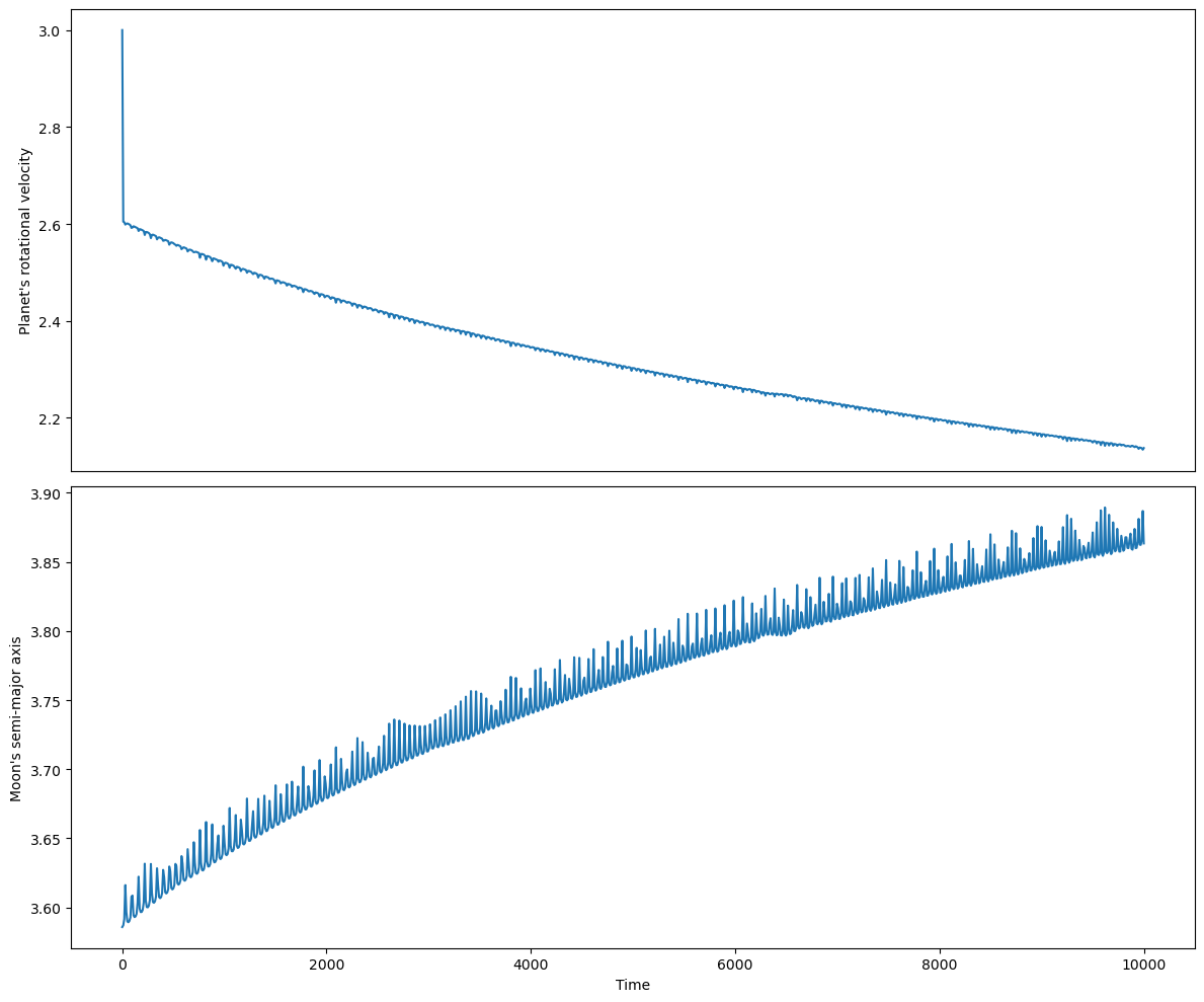
Leaving aside the big initial drop-off in the rotational velocity of the planet (which is due to the springs reacting to the high initial rotational velocity), we can see that indeed the long-term trend is the expected one: the planet’s rotation slows down and the moon’s orbit becomes wider.
Let us now flip things around by decreasing by a couple of orders of magnitude the initial rotational velocity of the planet:
ta.time = 0
ta.state[:] = 0
ta.state[2] = 5
ta.state[5 + N + 1] = -1.0 * mM / m0
ta.state[5 + N + 3] = 1
ta.state[5 + N + 4] = 0.03
out = ta.propagate_grid(time_grid)
r0_hist = out[-1][:, 0:2]
v0_hist = out[-1][:, 5 + N : 5 + N + 2]
rM_hist = out[-1][:, 2:4]
vM_hist = out[-1][:, 5 + N + 2 : 5 + N + 4]
alpha_hist = out[-1][:, 4]
valpha_hist = out[-1][:, 5 + N + 4]
l_hist = [out[-1][:, 5 + _] for _ in range(N)]
r_hist = [
r0_hist
+ np.array(
[
(a - l_hist[_]) * np.cos(alpha_hist + _ * (2.0 / N * np.pi)),
(a - l_hist[_]) * np.sin(alpha_hist + _ * (2.0 / N * np.pi)),
]
).transpose()
for _ in range(N)
]
a_hist = [
pykep.ic2par(
list(rM_hist[_] - r0_hist[_]) + [0],
list(vM_hist[_] - v0_hist[_]) + [0],
G * (m0 + sum(masses) + mM),
)[0]
for _ in range(len(r0_hist))
]
fig = plt.figure(figsize=(12, 10))
ax = plt.subplot(211)
plt.plot(time_grid, valpha_hist)
plt.ylabel("Planet's rotational velocity")
ax.set_xticks([])
plt.subplot(212)
plt.plot(time_grid, a_hist)
plt.xlabel("Time")
plt.ylabel("Moon's semi-major axis")
plt.tight_layout()
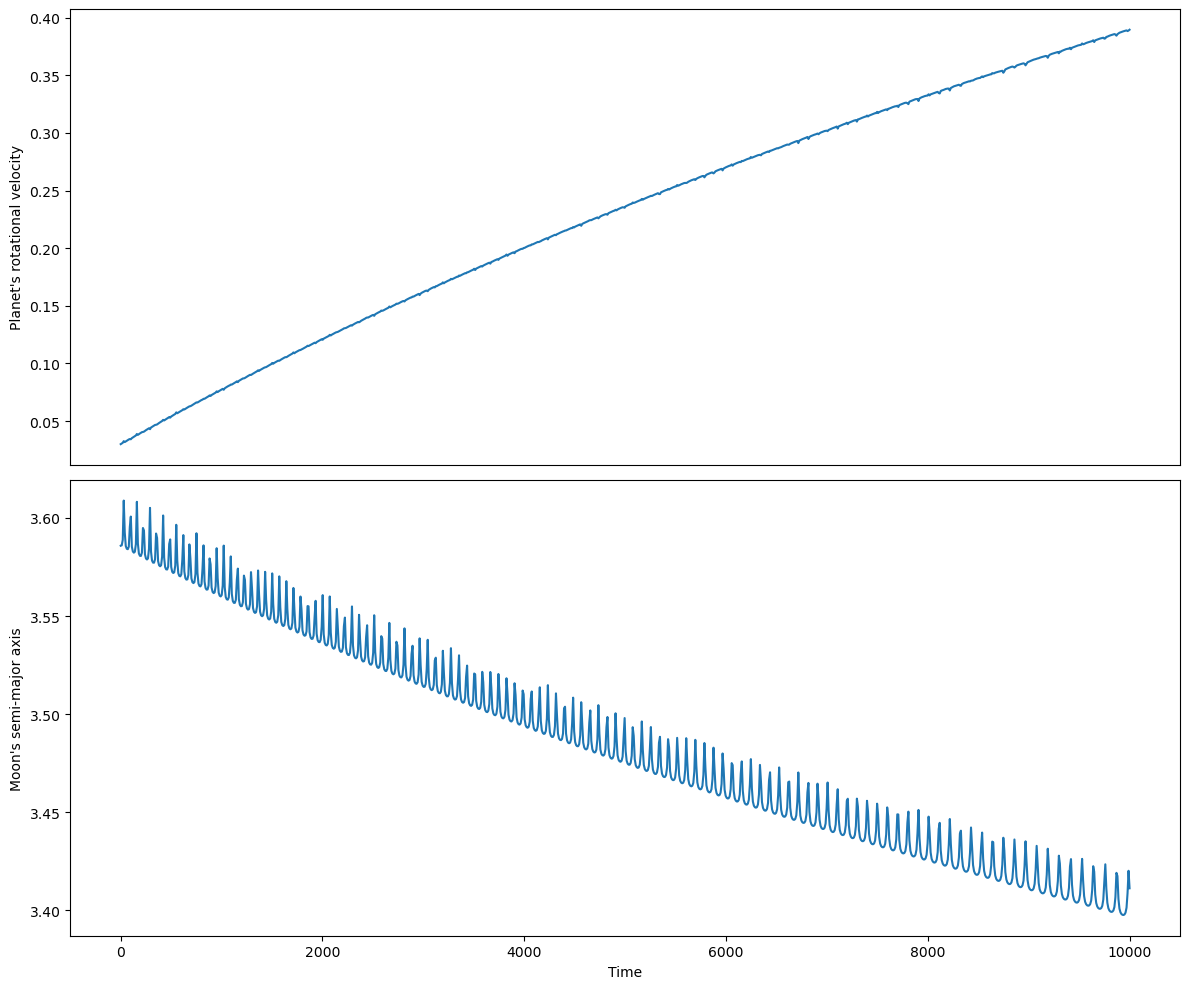
Indeed, as expected, the planet’s rotation accelerates while the moon’s orbit spirals inward.
As a last experiment, let us set up the moon in an almost-circular orbit whose period roughly coincides with the rotation period of the planet:
ta.time = 0
ta.state[:] = 0
ta.state[2] = 3.6
ta.state[5 + N + 1] = -1.892969448600091 * mM / m0
ta.state[5 + N + 3] = 1.892969448600091 * (1 - mM / m0)
ta.state[5 + N + 4] = 0.5258
out = ta.propagate_grid(time_grid)
r0_hist = out[-1][:, 0:2]
v0_hist = out[-1][:, 5 + N : 5 + N + 2]
rM_hist = out[-1][:, 2:4]
vM_hist = out[-1][:, 5 + N + 2 : 5 + N + 4]
alpha_hist = out[-1][:, 4]
valpha_hist = out[-1][:, 5 + N + 4]
l_hist = [out[-1][:, 5 + _] for _ in range(N)]
r_hist = [
r0_hist
+ np.array(
[
(a - l_hist[_]) * np.cos(alpha_hist + _ * (2.0 / N * np.pi)),
(a - l_hist[_]) * np.sin(alpha_hist + _ * (2.0 / N * np.pi)),
]
).transpose()
for _ in range(N)
]
a_hist = [
pykep.ic2par(
list(rM_hist[_] - r0_hist[_]) + [0],
list(vM_hist[_] - v0_hist[_]) + [0],
G * (m0 + sum(masses) + mM),
)[0]
for _ in range(len(r0_hist))
]
fig = plt.figure(figsize=(12, 10))
ax = plt.subplot(211)
plt.plot(time_grid, valpha_hist)
plt.ylabel("Planet's rotational velocity")
ax.set_xticks([])
plt.subplot(212)
plt.plot(time_grid, a_hist)
plt.xlabel("Time")
plt.ylabel("Moon's semi-major axis")
plt.tight_layout()
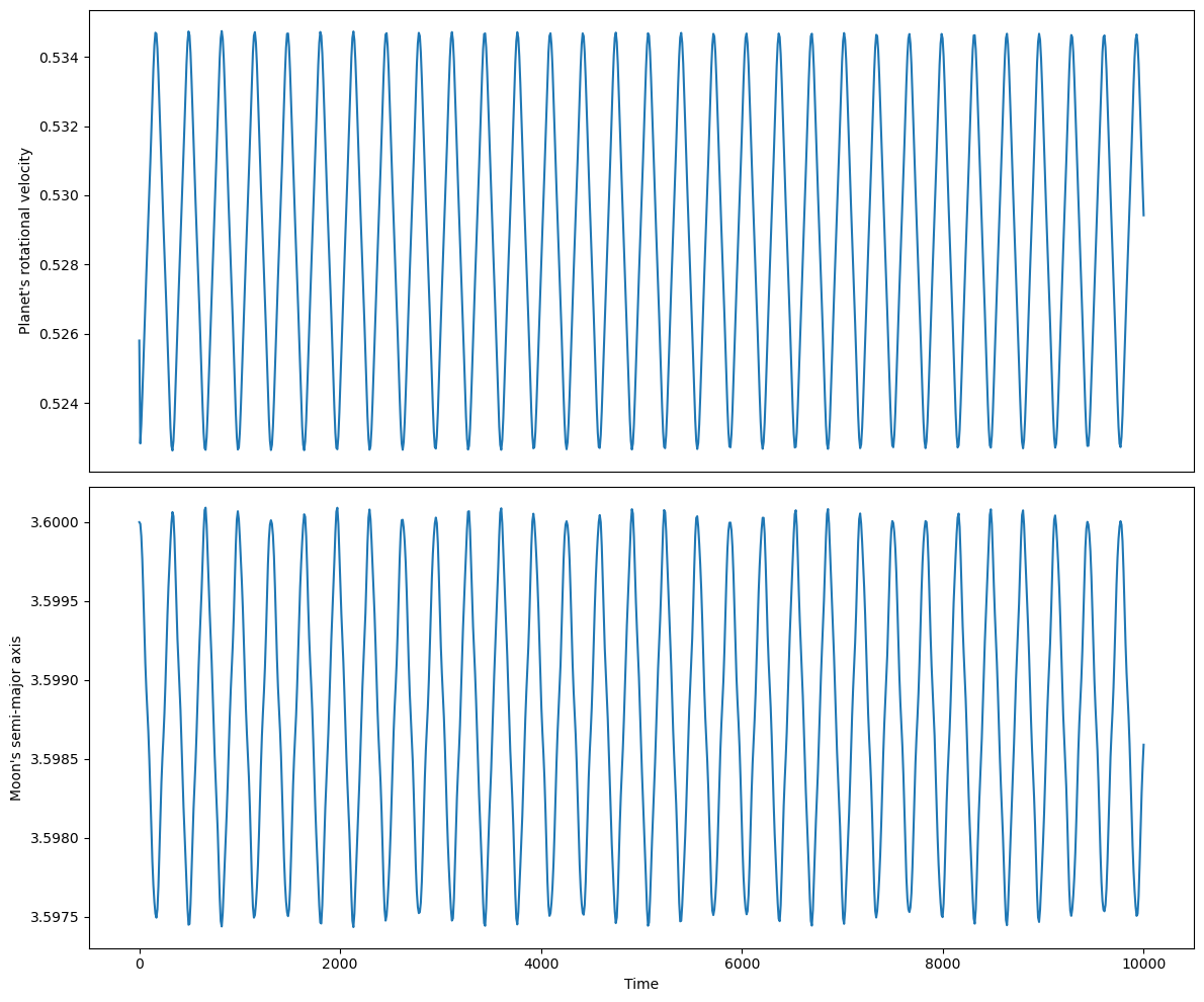
This synchronous configuration does not lead to a secular evolution in either the planet’s rotation or the moon’s orbital radius because the tidal bulge remains aligned to moon, rather than preceding or trailing it.
Analysing the bulge#
Lastly, we will attempt here a qualitative analysis of the tidal bulge’s behaviour. When the orbital period of the moon differs from the rotation period of the planet, the bulge raised by the tide will not be perfectly aligned with the moon, but it will either precede it (if the planet rotates faster than the moon’s orbit) or lag behind it (if the planet rotates slower than the moon’s orbit). Indeed, it is this misalignment which makes the secular evolution of the system possible by introducing a torque.
Let us begin by preparing the system with the moon in a near-circular orbit and the planet’s rotation period much smaller than the moon’s orbital period:
ta.time = 0
ta.state[:] = 0
ta.state[2] = 3.6
ta.state[5 + N + 1] = -1.892969448600091 * mM / m0
ta.state[5 + N + 3] = 1.892969448600091 * (1 - mM / m0)
ta.state[5 + N + 4] = 0.03
We can now integrate for a few time units:
time_grid = np.linspace(0, 200, 8000)
out = ta.propagate_grid(time_grid)
We will now proceed to create an animation visualising the evolution in time of the tidal bulge. Specifically, we place ourselves in the reference plane of the rotating planet and we amplify the values of the \(l_i\) coordinates in order to visually exaggerate the effect of the tides on the planet’s shape. The moon’s direction will be represented by a dashed grey line, which will be rotating counterclockwise. We will also be using the direction of the barycentre of the small masses \(m_i\) (represented by a dashed red line) as a rough indicator of the bulge’s orientation, which, in this setup, should be slightly lagging behind the moon.
Let us see:
%%capture
plt.rcParams["animation.embed_limit"] = 80
r0_hist = out[-1][:, 0:2]
rM_hist = out[-1][:, 2:4]
alpha_hist = out[-1][:, 4]
r_rel_hist = rM_hist - r0_hist
xM_rel_hist = r_rel_hist[:, 0] * np.cos(-alpha_hist) - r_rel_hist[:, 1] * np.sin(
-alpha_hist
)
yM_rel_hist = r_rel_hist[:, 0] * np.sin(-alpha_hist) + r_rel_hist[:, 1] * np.cos(
-alpha_hist
)
l_hist = [out[-1][:, 5 + _] for _ in range(N)]
r_hist = [
np.array(
[
(a - l_hist[_] * 100) * np.cos(_ * (2.0 / N * np.pi)),
(a - l_hist[_] * 100) * np.sin(_ * (2.0 / N * np.pi)),
]
).transpose()
for _ in range(N)
]
# Produce the animation.
fig = plt.figure(figsize=(8, 8))
ax = plt.subplot(111)
tcs = [plt.Circle((0.2, 0.0), 0.01, ec="black", fc="black", zorder=3) for _ in range(N)]
lns = [ax.plot([], [], "-", color="gray")[0] for _ in range(N)]
ln_rel = ax.plot([], [], "--", color="gray")[0]
ln_bar = ax.plot([], [], "--", color="red")[0]
(spl,) = ax.plot([], [], "-", color="orange")
for _ in tcs:
ax.add_artist(_)
ax.grid()
def init():
ax.set_xlim((-1.5, 1.5))
ax.set_ylim((-1.5, 1.5))
ax.set_aspect("equal")
return (*tcs, *lns, spl, ln_rel, ln_bar)
def animate(i):
i = i + 200
for _ in range(N):
tcs[_].set_center(r_hist[_][i])
bar = np.dot(np.array(masses), np.array(r_hist)[:, i]) / np.sum(masses)
bar_th = np.arctan2(bar[1], bar[0])
ln_bar.set_data([0, np.cos(bar_th)], [0, np.sin(bar_th)])
r_data = np.array([r_hist[_][i] for _ in range(N)] + [r_hist[0][i]])
tck, u = interpolate.splprep(r_data.transpose(), s=0, per=1)
unew = np.arange(0, 1.01, 0.001)
out = interpolate.splev(unew, tck)
spl.set_data(out[0], out[1])
for _ in range(N):
lns[_].set_data([0, r_hist[_][i, 0]], [0, r_hist[_][i, 1]])
ln_rel.set_data([0, xM_rel_hist[i]], [0, yM_rel_hist[i]])
return (*tcs, *lns, spl, ln_rel, ln_bar)
anim = HTML(
animation.FuncAnimation(
fig, animate, init_func=init, frames=1200, interval=50, blit=True
).to_jshtml()
)
anim