Interfacing torch to heyoka.py

Note

For an introduction on feed forward neural networks in heyoka.py, check out the example: Feed-Forward Neural Networks.

Warning

This tutorial assumes torch is installed

heyoka.py is not a library meant for machine learning, nor it aspires to be one. However, given its support for feed-forward neural networks and their potential use in numerical integration, it is useful to connect the heyoka.py ffnn() factory to a torch model. This tutorial tackles this!

import heyoka as hk

import numpy as np

# We will need torch for this notebook. The CPU version is enough though.
import torch
from torch import nn

We start defining a ffnn model in torch. We use as a test-case, a feed-forward neural network with two hidden layers having 32 neurons each and use tanh as nonlinearities and a sigmoid for the output layer. We define the model as to map it easily to the heyoka ffnn factory, but other styles are also possible.

This will typically look something like:

#Let us use float64 (this is not necessary as heyoka has also the float32 type, but we go for high precision here!)
torch.set_default_dtype(torch.float64)

class torch_net(nn.Module):
    def __init__(
        self,
        n_inputs=4,
        nn_hidden=[32, 32],
        n_out=1,
        activations=[nn.Tanh(), nn.Tanh(), nn.Sigmoid()]
    ):
        super(torch_net, self).__init__()

        # We treat all layers equally.
        dims = [n_inputs] + nn_hidden + [n_out]

        # Linear function.
        self.fcs = nn.ModuleList([nn.Linear(dims[i], dims[i + 1]) for i in range(len(dims) - 1)])

        # Non-linearities.
        self.acts = nn.ModuleList(activations)

    def forward(self, x):
        for fc, act in zip(self.fcs, self.acts):
            x = act(fc(x))
        return x

Weights and biases are stored by torch in the model as arrays, while heyoka flattens everything into a one-dimensional sequence containing all weights first, then all biases.

The following function takes care of converting the torch representation to heyoka’s:

def weights_and_biases_heyoka(model):
    weights = {}
    biases = {}

    for name, param in model.named_parameters():
        if 'weight' in name:
            weights[name] = param.data.clone()
        elif 'bias' in name:
            biases[name] = param.data.clone()
    biases_torch=[]
    weights_torch=[]
    for idx in range(len(weights)):
        weights_torch.append(weights[list(weights.keys())[idx]].numpy())
        biases_torch.append(biases[list(biases.keys())[idx]].numpy())
        
    w_flat=[]
    b_flat=[]
    for i in range(len(weights_torch)):
        w_flat+=list(weights_torch[i].flatten())
        b_flat+=list(biases_torch[i].flatten())
    w_flat=np.array(w_flat)
    b_flat=np.array(b_flat)
    print(w_flat.shape)
    return np.concatenate((w_flat, b_flat))

We are now ready to instantiate the model and extract its weights and biases ready for constructing an heyoka.ffnn object:

model = torch_net(n_inputs=4, 
                  nn_hidden=[32, 32],
                  n_out=1,
                  activations=[nn.Tanh(), nn.Tanh(), nn.Sigmoid()])

# Here one would likely perform some training ... at the end, we extract the model parameters:
flattened_weights = weights_and_biases_heyoka(model)

(1184,)

Let us instantiate the feed forward neural network in heyoka.py using those parameters:

inp_1, inp_2, inp_3, inp_4=hk.make_vars("inp_1","inp_2","inp_3","inp_4")
model_heyoka=hk.model.ffnn(inputs=[inp_1, inp_2, inp_3, inp_4], 
                           nn_hidden=[32,32], 
                           n_out=1,
                           activations=[hk.tanh,hk.tanh,hk.sigmoid], 
                           nn_wb=flattened_weights)

Good! Just to be sure, we now verify the output is the same at inference? Let’s first compile the network so that we can run inference:

model_heyoka_compiled=hk.cfunc(model_heyoka, [inp_1, inp_2, inp_3, inp_4])

… and create some random inputs

random_input=torch.rand((4,1000000))
random_input_torch=random_input.t()
random_input_numpy=random_input.numpy()
out_array=np.zeros((1,1000000))

Now, let’s compare the output of heyoka.ffnn and torch to see if they are identical

t_hey = model_heyoka_compiled(random_input_numpy,outputs=out_array)
t_torch = model(random_input_torch).detach().numpy().reshape(1,-1)

print("Maximum difference in the inference is: ", (t_hey-t_torch).max())

Maximum difference in the inference is:  1.1102230246251565e-16

In this way we have managed to port the torch model in heyoka.py, reproducing the same results…

Using torch optimizers

An some cases the parameters of the neural network may need to be updated with heyoka.py in the loop, check out the example: Neural ODEs.

This part shows how to interface with optimizers (in this case Adam) provided by torch.

In the following we use a simplified version of Neural ODEs, where a feedforward neural network learns the underlying dynamics of a liner system through observations.

import matplotlib.pylab as plt

Dynamics

\[ \left\{ \begin{array}{l} \dot x = Ax + b \end{array} \right. \]

# We now assemble the dynamics
A = np.array([
    [ 0. ,  0. ,  0. ,  1. ,  0. ,  0. ],
    [ 0. ,  0. ,  0. ,  0. ,  1. ,  0. ],
    [ 0. ,  0. ,  0. ,  0. ,  0. ,  1. ],
    [-2.5,  2. ,  0. ,  0. ,  0. ,  0. ],
    [ 2. , -5.4,  3.4,  0. ,  0. ,  0. ],
    [ 0. ,  3.4, -3.4,  0. ,  0. ,  0. ]
])

b = [0, 0, 0, -3.5, 0.26, 3.74]

n = len(b)
assert A.shape == (n, n)

x_vars = hk.make_vars(*[f"x_{i}" for i in range(1, n + 1)])

Ax_b =  A @ np.array(x_vars) + b
dynamics = list(zip(x_vars, Ax_b))

Setup

# This is the number of observations (i.e. the ground truth).
data_size = 1000
# This is the number of initial conditions to use in one batch (M)
batch_size_ic = 20
# This is the number of observations to predict from each sampled initial condition (T)
batch_size_time = 10
# This is the initial condition used to generate the observations (of the real dynamics)
ic = [2.0, 0.0, 0.0, 1.0, 0.0, 0.0]
# This is the time grid used to generate the observations
t_grid = np.linspace(0.0, 20, data_size)

The taylor integrator we use for the ground truth

ta = hk.taylor_adaptive(
    # The ODEs.
    dynamics,
    # The initial conditions.
    ic,
    # Operate in compact mode.
    compact_mode=False,
    # Define the tolerance
    tol=1e-18,
)

We generate the ground truth (observations)

ta.time = 0
ta.state[:] = ic
gt = ta.propagate_grid(t_grid)[5]

# Visualize
def plot_t_evol(out, tgrid, labels, title="", color='#1f77b4', batchy=None, tgrid_batch=None, color_batch=None, batch_ic=None, t_grids=None, ta_var=None, ic_var=None, nn_wb=None, batch_t_grid=None):
    fig = plt.figure(figsize = (12, 6))

    if len(title) > 0:
        fig.suptitle(title)
    
    ncoord = out.shape[1]
    ncols = 3
    nrows = ncoord // ncols + (ncoord % ncols)

    for i in range(0, ncoord):
        ax = fig.add_subplot(nrows, ncols, i + 1)
        ax.plot(tgrid, out[:, i], color=color)

        if batchy is not None:
            for j, t_grid_batch in enumerate(tgrid_batch):
                ax.plot(t_grid_batch, batchy[:,j,i], linewidth=3, color=color_batch)

        if batch_ic is not None:
            for one_ic, t_grid_batch in zip(batch_ic, t_grids):
                ta_var.time=0
                ta_var.state[:] = list(one_ic) + ic_var
                ta_var.pars[:] = nn_wb
                sol = ta_var.propagate_grid(batch_t_grid)[5]
                ax.plot(t_grid_batch, sol[:,i], linewidth=3, marker=".", color="#ff7f0e")

        ax.set_xlabel("Time [-]")
        ax.set_ylabel(labels[i], rotation=0, labelpad=10)
    
    plt.tight_layout()

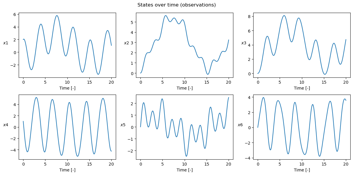
plot_t_evol(gt, t_grid, 
            ["$x1$", "$x2$", "$x3$", "$x4$", "$x5$", "$x6$"], 
            title="States over time (observations)")

This creates the batch.

def get_batch(t_data, x_data, batch_size_ic, batch_size_time):
    # We select the initial conditions from which generate predictions
    s = np.random.choice(
        np.arange(gt.shape[0] - batch_size_time, dtype=np.int64),
        batch_size_ic,
        replace=False,
    )
    ic_batch = x_data[s, :]  # (M, n)
    # Assuming uniform grid and a non-autonomous system, all predictions will be made on the same time grid
    t_batch = t_data[:batch_size_time]  # (T)
    t_grids = np.array([t_data[s_:s_+batch_size_time] for s_ in s])  # Used for plotting
    x_batch = np.stack([x_data[s + i] for i in range(batch_size_time)])  # (T, M, n)
    return ic_batch, t_batch, x_batch, t_grids

This instantiates the ffnn as heyoka expression, and defines the neural ODE

# We define as nonlinearity a simple linear layer
linear = lambda inp: inp

# We call the factory to construct a FFNN. Following the torcheqdiff example here we put cubes as inputs:
ffnn = hk.model.ffnn(
    inputs=x_vars,
    nn_hidden=[30, 30],
    n_out=len(x_vars),
    activations=[hk.tanh, hk.tanh, linear]
)

# We thus define the neural dynamics
dyn_n = list(zip(x_vars, ffnn))

We now need the gradient of the loss over the batch

\[ \mathcal L_{\theta} = \sum_{i=0}^{M}\sum_{j=0}^T (\pmb y_{ij} - \hat {\pmb y}_{ij})\cdot (\pmb y_{ij} - \hat {\pmb y}_{ij}) \]

\[ \frac{\partial L_\theta}{\partial \theta} = 2 \sum_{i=0}^{M}\sum_{j=0}^T (\pmb y_{ij} - \hat {\pmb y}_{ij})\cdot \frac{\partial \pmb y_{ij}}{\partial \theta} \]

hence we need a variational integrator.

var_dyn_n = hk.var_ode_sys(dyn_n, args = hk.var_args.params)
ta_var = hk.taylor_adaptive(
    # The ODEs.
    var_dyn_n,
    # The initial conditions.
    ic,
    # Operate in compact mode.
    compact_mode=True,
    # Define the tolerance
    tol=1e-8,
)
# We store for convenience the initial conditions of the variational state
ic_var = list(ta_var.state[n:])

batch_ic, batch_t_grid, batch_y, t_grids = get_batch(t_grid, gt, batch_size_ic, batch_size_time)

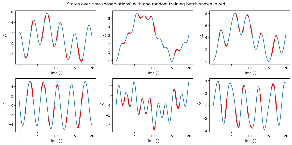
plot_t_evol(gt, t_grid, 
            ["$x1$", "$x2$", "$x3$", "$x4$", "$x5$", "$x6$"], 
            title="States over time (observations) with one random training batch shown in red", 
            batchy=batch_y, tgrid_batch=t_grids, color_batch='red')

# We find initialization values for weigths / biases
n_pars = len(ta_var.pars)
nn_wb = np.random.normal(loc = 0, scale = 0.1, size = (n_pars, ))

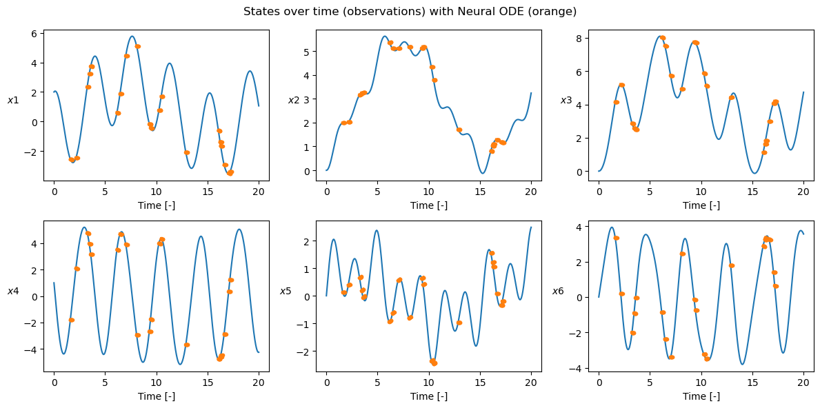
plot_t_evol(gt, t_grid, 
            ["$x1$", "$x2$", "$x3$", "$x4$", "$x5$", "$x6$"], 
            title="States over time (observations) with Neural ODE (orange)", 
            batch_ic=batch_ic, t_grids=t_grids, ta_var=ta_var, ic_var=ic_var, nn_wb=nn_wb, batch_t_grid=batch_t_grid)

This returns the value of the loss and gradients of the loss with respect to the network parameters

def loss_and_gradient(nn_wb, batch_ic, batch_y):
    # We loop over the various selected initial conditions and produce the predictions
    # and their gradients
    # We reset the batch_loss value
    batch_loss = 0
    # We reset the gradient loss
    grad = np.array([0.] * len(ta_var.pars))
    for i, ic_ in enumerate(batch_ic):
        ta_var.time=0
        ta_var.state[:] = list(ic_) + ic_var
        ta_var.pars[:] = nn_wb
        sol = ta_var.propagate_grid(batch_t_grid)[5]
        # Here is the term (y-y_hat)
        diff = (sol[:,:n] - batch_y[:,i,:])
        # Which is now summed sum sum (y-y_hat).(y-y_hat)
        batch_loss += np.sum(diff**2)
        # And the gradient computed  as 2 sum (y-y_hat).dy
        for dy in sol[:,n:].reshape(batch_y.shape[0],n,-1):
            grad += 2*np.sum(diff@dy, axis=0)
    # We then take the mean over the points used
    batch_loss /= (batch_size_ic * batch_size_time)
    grad /= (batch_size_ic * batch_size_time)
    return batch_loss, grad

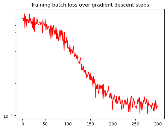
Simple fixed learning rate stochastic gradient descent

# We create a random batch
batch_losses = []
learning_rate = 1e-2

for i in range(300):
    batch_ic, batch_t_grid, batch_y, _ = get_batch(t_grid, gt, batch_size_ic=20, batch_size_time=10)
    batch_loss, grad = loss_and_gradient(nn_wb, batch_ic, batch_y)
    print(f"iter: {i}, loss : {batch_loss:.3e}", end="\r")
    nn_wb = nn_wb - learning_rate * grad
    batch_losses.append(batch_loss)

iter: 299, loss : 1.220e-01

plt.semilogy(batch_losses, color="red")
plt.title("Training batch loss over gradient descent steps")

Text(0.5, 1.0, 'Training batch loss over gradient descent steps')

ta_var.time = 0
ta_var.state[:] = ic + ic_var
ta_var.pars[:] = nn_wb
sol = ta_var.propagate_grid(t_grid)[5]

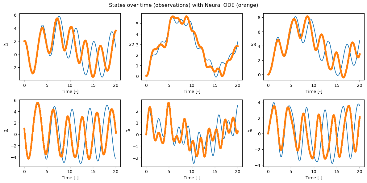
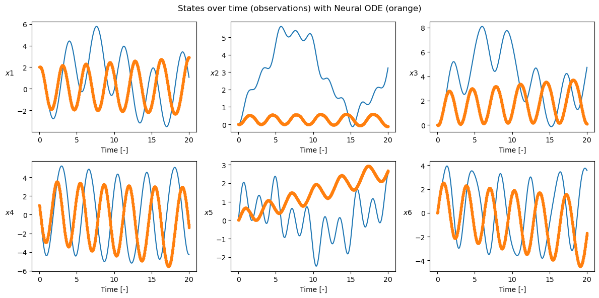
plot_t_evol(gt, t_grid, 
            ["$x1$", "$x2$", "$x3$", "$x4$", "$x5$", "$x6$"], 
            title="States over time (observations) with Neural ODE (orange)", 
            batch_ic=[ic], t_grids=[t_grid], ta_var=ta_var, ic_var=ic_var, nn_wb=nn_wb, batch_t_grid=t_grid)

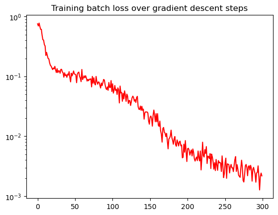
Now we do the same training with the Adam Optimizer

# Reinitialize values for weigths / biases
n_pars = len(ta_var.pars)
nn_wb = np.random.normal(loc = 0, scale = 0.1, size = (n_pars, ))

# Set desired precision
precision = np.single # np.double
learning_rate = 1e-2

# Determine the PyTorch dtype based on precision
dtype = torch.float32 if precision == np.single else torch.float64

# Gradient descent using the Adam optimizer 
weights_biases_tensor = torch.tensor(nn_wb, dtype= dtype, requires_grad=True)
optimizer = torch.optim.Adam([weights_biases_tensor], lr=precision(learning_rate), betas=(0.9, 0.999), eps=precision(1e-8), amsgrad=True)

# We create a random batch
batch_losses = []

for i in range(300):
    batch_ic, batch_t_grid, batch_y, _ = get_batch(t_grid, gt, batch_size_ic=20, batch_size_time=10)
    batch_loss, grad = loss_and_gradient(nn_wb, batch_ic, batch_y)
    print(f"iter: {i}, loss : {batch_loss:.3e}", end="\r")
    batch_losses.append(batch_loss)

    # Clear the gradients for the next iteration
    optimizer.zero_grad()

    # weights_biases_tensor.data = torch.tensor(current_weights)
    weights_biases_tensor.data = torch.tensor(np.array(nn_wb), dtype=dtype, requires_grad=True)
    
    # Convert to tensor
    dLdw_tensor = torch.tensor(np.squeeze(grad), dtype=dtype)

    # Manually set the gradients for the parameter
    weights_biases_tensor.grad = dLdw_tensor

    # Use the Adam optimizer to perform the weight update
    optimizer.step()

    # Convert back to array
    nn_wb = weights_biases_tensor.detach().numpy()

iter: 299, loss : 2.181e-03

plt.semilogy(batch_losses, color="red")
plt.title("Training batch loss over gradient descent steps")

Text(0.5, 1.0, 'Training batch loss over gradient descent steps')

ta_var.time = 0
ta_var.state[:] = ic + ic_var
ta_var.pars[:] = nn_wb
sol = ta_var.propagate_grid(t_grid)[5]

plot_t_evol(gt, t_grid, 
            ["$x1$", "$x2$", "$x3$", "$x4$", "$x5$", "$x6$"], 
            title="States over time (observations) with Neural ODE (orange)", 
            batch_ic=[ic], t_grids=[t_grid], ta_var=ta_var, ic_var=ic_var, nn_wb=nn_wb, batch_t_grid=t_grid)