Non-autonomous systems

All the ODE systems we have used in the examples thus far belong to the class of autonomous systems. That is, the time variable \(t\) never appears explicitly in the expressions of the right-hand sides of the ODEs. In this section, we will see how non-autonomous systems can be defined and integrated in heyoka.py.

The dynamical system we will be focusing on is, again, a pendulum, but this time we will spice things up a little by introducing a velocity-dependent damping effect and a time-dependent external forcing. These additional effects create a rich and complex dynamical picture which is highly sensitive to the initial conditions. See here for a detailed analysis of this dynamical system.

The ODE system of the forced damped pendulum reads:

\[\begin{split} \begin{cases} x^\prime = v \\ v^\prime = \cos t - 0.1v - \sin(x) \end{cases}. \end{split}\]

The \(\cos t\) term represents a periodic time-dependent forcing, while \(-0.1v\) is a linear drag representing the effect of air on the pendulum’s bob. We take as initial conditions

\[\begin{split} \begin{cases} x\left( 0 \right) = 0 \\ v\left( 0 \right) = 1.85 \end{cases}. \end{split}\]

That is, the pendulum is initially in the vertical position with a positive velocity.

The time variable is represented in heyoka.py’s expression system by a special placeholder called, in a dizzying display of inventiveness, time. Because the name time is fairly common, it is generally a good idea to prepend the module name heyoka (or its usual abbreviation, hy) when using the time expression, in order to avoid ambiguities. With that in mind, let’s look at how the forced damped pendulum is defined in heyoka.py:

import heyoka as hy

# Create the symbolic variables x and v.
x, v = hy.make_vars("x", "v")

# Create the integrator object.
ta = hy.taylor_adaptive(
                        # Definition of the ODE system:
                        # x' = v
                        # v' = cos(t) - 0.1*v - sin(x)
                        sys = [(x, v),
                         (v, hy.cos(hy.time) - .1 * v - hy.sin(x))],
                        # Initial conditions for x and v.
                        state = [0., 1.85],
                        # Explicitly specify the
                        # initial value for the time
                        # variable.
                        time = 0.
                        )

ta

C++ datatype            : double
Tolerance               : 2.220446049250313e-16
High accuracy           : false
Compact mode            : false
Taylor order            : 20
Dimension               : 2
Time                    : 0
State                   : [0, 1.85]

Note that, for the sake of completeness, we passed an explicit initial value for the time variable via the keyword argument time. In this specific case, this is superfluous, as the default initial value for the time variable is already zero.

We can now integrate the system for a few time units, checking how the value of \(x\) varies in time:

import numpy as np
from matplotlib.pylab import plt

fig = plt.figure(figsize=(12,6))

# Construct a time grid from t=0 to t=200.
t_grid = np.linspace(0, 200, 1000)

# Propagate over the time grid.
x_hist = ta.propagate_grid(t_grid)[5][:,0]

# Display the time evolution for the x variable.
plt.plot(t_grid, x_hist)
plt.xlabel("Time")
plt.ylabel("x");

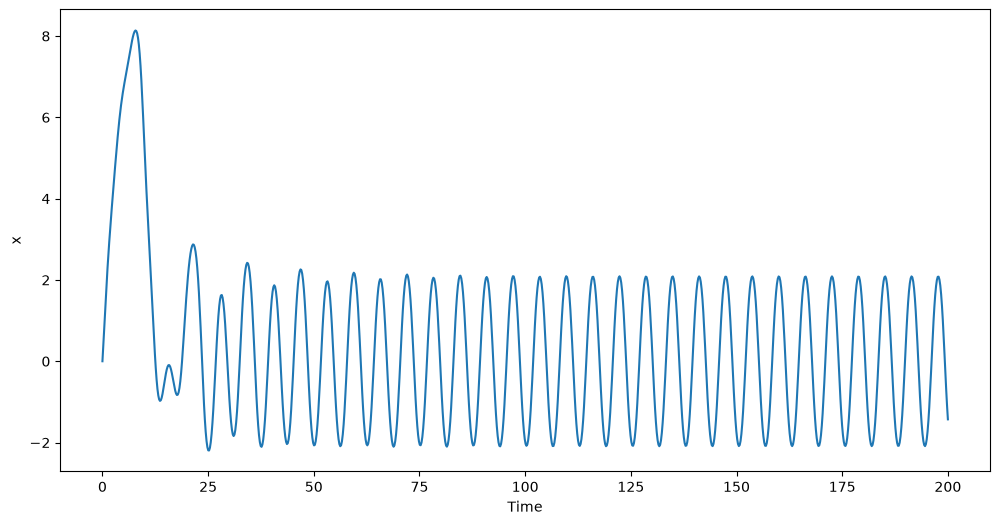
After an initial excursion to higher values for \(x\), the system seems to settle into a stable motion. Note that, because this system can exhibit chaotic behaviour, changing the initial conditions by a small amount might lead to a qualitatively-different long-term behaviour.