The Tolman–Oppenheimer–Volkoff equations (Lindblom’s form)#
We study the log-entalpy formulation of the Oppenheimer–Volkoff equations (also known as Lindblom’s form). This formulation (here taken from Martin Jakob Steil’s thesis in Section 3.2.3) has several advantages w.r.t. the original formulation by Tolman–Oppenheimer–Volkoff:
It directly describes the radius and mass of the star.
It has a known integration domain.
It is not stiff.
In this formulation, the state is:
and the parameters are:
where \(K = \overline K(1+\eta_K)\) and \(\Gamma = \overline \Gamma(1+\eta_\Gamma)\) will parameterize the equation of state of a polytrope (a gaseous sphere in hydrodynamic equilibrium).
The equations are then written as:
where an equation of state is needed to define the pressure \(P(h)\) and energy density \(\epsilon(h)\) expressions.
In the case of a relativistic polytrope here studied, the log-entalpy is introduced and defined as:
where \(\rho\) is the (baryonic) mass density (following a polytropic process):
Hence, in this case the log-entalpy can be written as:
which can be inverted to yield the \(P(h)\) form:
Note: the dynamics is singular at \(h=0\) (of a removable kind), so we will need to define the initial conditions at some small \(\delta h\) where the singularity is not present.
import heyoka as hy
import numpy as np
from scipy import optimize
from copy import deepcopy

import time

import matplotlib.pyplot as plt
Preamble#
Let us start by introducing common definitions and the reference numerical values we will be using for the parameters \(K, \Gamma\) of the polytrope.
# State variables
x0, x1 = hy.make_vars("x0", "x1")

# The independent variable is log-enthalpy not time, thus we rename it as follows:
h = hy.time

# Parameters values
Gamma_v = 2.0
K_v = 100.0

# Parameters expressions
Gamma = Gamma_v * (1.0 + hy.par[0])
K = K_v * (1.0 + hy.par[1])

# Other expressions
P = K ** (-1.0 / (Gamma - 1.0)) * ((Gamma - 1.0) / Gamma * (hy.exp(h) - 1.0)) ** (
    Gamma / (Gamma - 1.0)
)
rho = (P / K) ** (1.0 / Gamma)
eps = rho + P / (Gamma - 1.0)

# The dynamics
dx0dh = -2.0 * x0 * (1.0 - 2.0 * x1) / (4.0 * np.pi * x0 * P + x1)
dyn = [
    (x0, dx0dh),
    (x1, (2.0 * np.pi * eps - x1 / 2.0 / x0) * dx0dh),
]
Standard Numerical Solution#
The Tolman–Oppenheimer–Volkoff equations in the Lindblom form are numerically well behaved.
We here show a straightforward numerical integration using the Taylor adaptive scheme of heyoka.
# We instantiate the numerical ODE solver
ta = hy.taylor_adaptive(dyn, state=[1.0, 1.0], time=0.1, tol=1e-16)
We define the conditions at the star center fixing the pressure \(P_c\), and thus computing the corresponding density \(\rho_c\), energy density \(\epsilon_c\) and log-entalpy \(h_c\)
# Pressure (change this value to then approximate different part of the M-R curve)
P_c = 1e-2

# Density
rho_c = (P_c / K_v) ** (1.0 / Gamma_v)

# Energy density
eps_c = rho_c + P_c / (Gamma_v - 1.0)

# log-entalpy
h_c = np.log(
    1 + Gamma_v / (Gamma_v - 1) * K_v ** (1 / Gamma_v) * P_c ** (1.0 - 1.0 / Gamma_v)
)

print("Conditions at the star center:")
print("\nPressure: ", P_c)
print("Energy density: ", eps_c)
print("Density: ", rho_c)
print("log-entalpy: ", h_c)
Conditions at the star center:

Pressure:  0.01
Energy density:  0.02
Density:  0.01
log-entalpy:  1.0986122886681098
From the conditions at the star center (c) we derive the initial conditions (0) for the numerical integration offsetting the entalpy (the independent variable) by a small amount, thus avoiding the numerical (removable) singularity in the dynamics:
# Since the dynamics is singular at h_c, we define the initial conditions at h_0 = h_c - dh
dh = 1e-6  # note that if this gets too small the variational equations may have numerical issues at h_0.
h_0 = h_c - dh

# Initial conditions at h_0 (from Steil thesis). Could be improved at second order.
x0_0 = 3.0 / (2.0 * np.pi * (3.0 * P_c + eps_c)) * dh
x1_0 = 2.0 * eps_c / (3 * P_c + eps_c) * dh
y_0 = [x0_0, x1_0]
We are now ready to perform a numerical integration, and extract from the result the star radius and mass:
start = time.time()
ta.time = h_0
ta.state[:] = y_0
ta.pars[:] = [0.0, 0.0]
time_grid = np.linspace(h_0, 0.0, 100)
sol = ta.propagate_grid(time_grid)
time_cost = time.time() - start
print("Total time to propagate:", time_cost)
print("Outcome (should be time_limit if all went well): ", str(sol[0]).split(".")[1])

# The mass and radius are easily computed from the last value reached
rf = np.sqrt(sol[-1][:, 0][-1])
Mf = sol[-1][:, 1][-1] * rf

print("Final value for the stellar radius is: ", rf)
print("Final value for the stellar mass is: ", Mf)
Total time to propagate: 0.00038123130798339844
Outcome (should be time_limit if all went well):  time_limit
Final value for the stellar radius is:  5.511134830596981
Final value for the stellar mass is:  1.3684613613885503
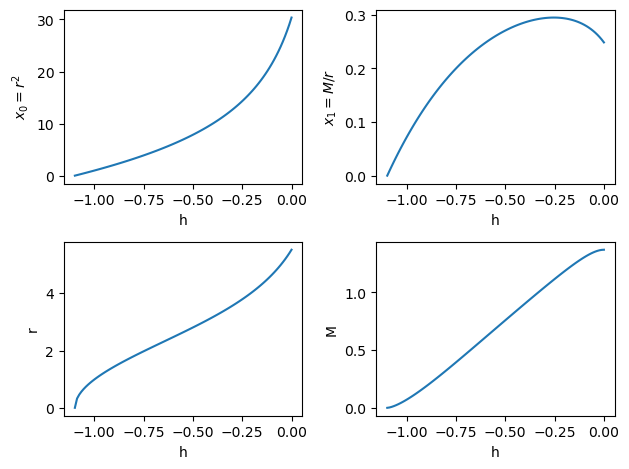
we now plot the results of the numerical integration.
r2_plot = sol[-1][:, 0]
mr_plot = sol[-1][:, 1]

# Plots
ax = plt.subplot(2, 2, 1)
ax.plot(-time_grid, r2_plot)
ax.set_xlabel("h")
ax.set_ylabel("$x_0 = r^2$")

ax = plt.subplot(2, 2, 2)
ax.plot(-time_grid, mr_plot)
ax.set_xlabel("h")
ax.set_ylabel("$x_1 = M / r$")

ax = plt.subplot(2, 2, 3)
ax.plot(-time_grid, np.sqrt(r2_plot))
ax.set_xlabel("h")
ax.set_ylabel("r")

ax = plt.subplot(2, 2, 4)
ax.plot(-time_grid, mr_plot * np.sqrt(r2_plot))
ax.set_xlabel("h")
ax.set_ylabel("M")
plt.tight_layout()
Variational equations#
We seek an analytical expression for the stellar mass and radius, as a function of the variation of the conditions at the stellar center \(\delta h_c\).
In order to obtain the expressions seeked, a variational equation for the initial value of the entalpy (the independent variable) \(h_0\) is also needed. We thus introduce a last variable change \(\overline h_0 s = h\) so that the differential equations become:
with:
and:
and must be integrated for \(s \in [1, 0]\), which will correspond to \(h \in [\overline h_0, 0]\).
# The independent variable is s, not h = log(entalpy) nor t.
s = hy.time

# Important expressions
P = K ** (-1.0 / (Gamma - 1.0)) * (
    (Gamma - 1.0) / Gamma * (hy.exp(hy.par[2] * s) - 1.0)
) ** (Gamma / (Gamma - 1.0))
rho = (P / K) ** (1.0 / Gamma)
eps = rho + P / (Gamma - 1.0)

# We define the dynamics
dx0ds = (-2.0 * x0 * (1.0 - 2.0 * x1) / (4.0 * np.pi * x0 * P + x1)) * hy.par[2]
dyn2 = [
    (x0, dx0ds),
    (x1, (2.0 * np.pi * eps - x1 / 2.0 / x0) * dx0ds),
]
# We augment the dynamics with the variational equations (we use 8th order but lower orders are good already)
var_sys = hy.var_ode_sys(dyn2, args=[x0, x1, hy.par[2]], order=8)

# We instantiate the Taylor adaptive integrator for the system of equations augmented with the variational ones
ta_var = hy.taylor_adaptive(
    var_sys,
    state=[1.0, 1.0],
    time=0.1,
    tol=1e-18,
    compact_mode=True,
)
# We copy, for future reference, the initial conditions on the variational state
ic_var = list(deepcopy(ta_var.state[2:]))
start = time.time()
ta_var.time = 1.0

ta_var.state[:] = y_0 + ic_var
ta_var.pars[:] = [0.0, 0.0, h_0]

s_grid = np.linspace(1.0, 0.0, 100)
sol_var = ta_var.propagate_grid(s_grid)
print("Total time to propagate:", time.time() - start)
print("Outcome: ", sol_var[0])

rf = np.sqrt(sol_var[-1][:, 0][-1])
Mf = sol_var[-1][:, 1][-1] * rf

print("Final value for the stellar radius is: ", rf)
print("Final value for the stellar mass is: ", Mf)
Total time to propagate: 13.353347539901733
Outcome:  taylor_outcome.time_limit
Final value for the stellar radius is:  5.51113483059698
Final value for the stellar mass is:  1.3684613613885492
We have thus computed the following polynomial approximations (degree \(k\)):
Note the underscript \(0\) refers to the initial values, not to the star center which would here be indicated using \(c\) rather than \(0\).
# We repeat the computation changing the pressure at the center.

# Pressure
P_c_new = P_c * (1.0 + 3.0)

# Density
rho_c_new = (P_c_new / K_v) ** (1.0 / Gamma_v)

# Energy density
eps_c_new = rho_c_new + P_c_new / (Gamma_v - 1.0)

# log-entalpy
h_c_new = np.log(
    1
    + Gamma_v / (Gamma_v - 1) * K_v ** (1 / Gamma_v) * P_c_new ** (1.0 - 1.0 / Gamma_v)
)

print("Conditions at the star center:")
print("\nPressure: ", P_c_new)
print("Energy density: ", eps_c_new)
print("Density: ", rho_c_new)
print("log-entalpy: ", h_c_new)
Conditions at the star center:

Pressure:  0.04
Energy density:  0.06
Density:  0.02
log-entalpy:  1.6094379124341003
We may now find the new starting conditions at \(h_c-dh\).
h_0_new = h_c_new - dh

# Initial conditions at h_0_new (from Steil thesis). Can be improved at second order.
x0_0_new = 3.0 / (2.0 * np.pi * (3.0 * P_c_new + eps_c_new)) * dh
x1_0_new = 2.0 * eps_c_new / (3 * P_c_new + eps_c_new) * dh
y_0_new = [x0_0_new, x1_0_new]
We can now use the Taylor approximation to compute the stellar radius and mass:
taylor_approx = ta_var.eval_taylor_map(
    [x0_0_new - x0_0, x1_0_new - x1_0, h_0_new - h_0]
)
rf_new_taylor = np.sqrt(taylor_approx[0])
Mf_new_taylor = taylor_approx[1] * rf_new_taylor

print("Final value for the stellar radius is: ", rf_new_taylor)
print("Final value for the stellar mass is: ", Mf_new_taylor)
Final value for the stellar radius is:  4.902302695454508
Final value for the stellar mass is:  1.1364855355000758
We now compute these values by numerical integration.
start = time.time()
ta.time = h_0_new
ta.state[:] = y_0_new
ta.pars[:] = [0.0, 0.0]
time_grid = np.linspace(h_0_new, 0.0, 100)
sol_new = ta.propagate_grid(time_grid)
time_cost = time.time() - start
print("Total time to propagate:", time_cost)
print(
    "Outcome (should be time_limit if all went well): ", str(sol_new[0]).split(".")[1]
)

# The mass and radius are easily computed from the last value reached
rf_new = np.sqrt(sol_new[-1][:, 0][-1])
Mf_new = sol_new[-1][:, 1][-1] * rf_new

print("Final value for the stellar radius is: ", rf_new)
print("Final value for the stellar mass is: ", Mf_new)
Total time to propagate: 0.0002846717834472656
Outcome (should be time_limit if all went well):  time_limit
Final value for the stellar radius is:  4.9020827509255644
Final value for the stellar mass is:  1.13645940407093
Lets see the error introduced by the Taylor approximation in this specific instance:
print("Absolute error on mass:", Mf_new - Mf_new_taylor)
print("Absolute error on radius:", rf_new - rf_new_taylor)

print("\nRelative error on mass:", (Mf_new - Mf_new_taylor) / Mf_new)
print("Relative error on radius:", (rf_new - rf_new_taylor) / rf_new)
Absolute error on mass: -2.61314291458703e-05
Absolute error on radius: -0.00021994452894347205

Relative error on mass: -2.299371983923445e-05
Relative error on radius: -4.486756754604851e-05
The \(M_\odot\) vs \(R_\odot\) plot#
We now loop over different star conditions (at the core) and plot the relation between mass and radius using the Taylor approximation and the numerical integrator.
start = time.time()
Rstar = []
Mstar = []
P_grid = np.linspace(P_c * (1.0 - 0.95), P_c * (1 + 20.0), 1000)
for P_c_new in P_grid:
    # Density
    rho_c_new = (P_c_new / K_v) ** (1.0 / Gamma_v)

    # Energy density
    eps_c_new = rho_c_new + P_c_new / (Gamma_v - 1.0)

    # log-entalpy
    h_c_new = np.log(
        1
        + Gamma_v
        / (Gamma_v - 1)
        * K_v ** (1 / Gamma_v)
        * P_c_new ** (1.0 - 1.0 / Gamma_v)
    )

    # Since the dynamics is singular at h_c, we define the initial conditions at h_0 = h_c - dh
    h_0_new = h_c_new - dh

    # Initial conditions at h_0 (from Steil thesis). Can be improved at second order.
    x0_0_new = 3.0 / (2.0 * np.pi * (3.0 * P_c_new + eps_c_new)) * dh
    x1_0_new = 2.0 * eps_c_new / (3 * P_c_new + eps_c_new) * dh
    taylor_approx = ta_var.eval_taylor_map(
        [x0_0_new - x0_0, x1_0_new - x1_0, h_0_new - h_0]
    )
    Rstar.append(np.sqrt(taylor_approx[0]))
    Mstar.append(taylor_approx[1] * np.sqrt(taylor_approx[0]))
time_cost = time.time() - start
print("Total computation time using the Taylor Map:", time_cost)
Total computation time using the Taylor Map: 0.0064754486083984375
start = time.time()
Rstar_gt = []
Mstar_gt = []
P_grid = P_c * np.logspace(0.01, 12, 1000) / 40.0
for P_c_new in P_grid:
    # Density
    rho_c_new = (P_c_new / K_v) ** (1.0 / Gamma_v)

    # Energy density
    eps_c_new = rho_c_new + P_c_new / (Gamma_v - 1.0)

    # log-entalpy
    h_c_new = np.log(
        1
        + Gamma_v
        / (Gamma_v - 1)
        * K_v ** (1 / Gamma_v)
        * P_c_new ** (1.0 - 1.0 / Gamma_v)
    )

    # Since the dynamics is singular at h_c, we define the initial conditions at h_0 = h_c - dh
    h_0_new = h_c_new - dh

    # Since the dynamics is singular at h_c, we define the initial conditions at h_0 = h_c - dh
    h_0_new = h_c_new - dh

    # Initial conditions at h_0 (from Steil thesis). Can be improved at second order.
    x0_0_new = 3.0 / (2.0 * np.pi * (3.0 * P_c_new + eps_c_new)) * dh
    x1_0_new = 2.0 * eps_c_new / (3 * P_c_new + eps_c_new) * dh

    ta.time = h_0_new
    ta.state[:] = y_0_new
    outcome = ta.propagate_until(0.0)

    # The mass and radius are easily computed from the last value reached
    Rstar_gt.append(np.sqrt(ta.state[0]))
    Mstar_gt.append(ta.state[1] * np.sqrt(ta.state[0]))
time_cost = time.time() - start
print("Total time using the numerical integrator:", time_cost)
Total time using the numerical integrator: 0.10077452659606934
And lets have a look at the difference in the computed values for this range:
plt.plot(Rstar_gt, Mstar_gt, label="Ground truth")
plt.plot(Rstar, Mstar, c="r", alpha=0.5, label="Taylor Map (order 8)")

plt.xlabel(r"$R_{\odot}$")
plt.ylabel(r"$M_{\odot}$")
plt.legend()
<matplotlib.legend.Legend at 0x7fa4d7f1b0b0>
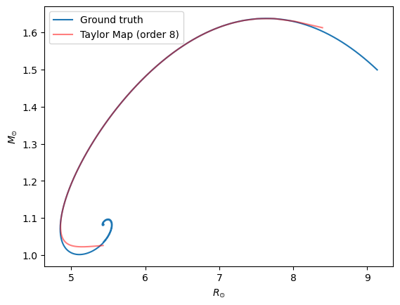
Conclusions:
the use of the high order variational equations to solve the Tolman–Oppenheimer–Volkoff equations result in a relatively large convergence radius (when using the Lindblom form) of the resulting Taylor map.
the resulting speedup in the evaluation of the mass/radius curve seems to be of the order of one order of magnitude.
the Taylor map allows to capture well the maximum allowed stellar mass.
We are not sure this is useful, but damn its cool!