The EGM2008 model#
Added in version 7.3.0.
heyoka.py includes an implementation of the EGM2008 geopotential model, enabling precise calculations of Earth’s gravitational potential and acceleration. This is essential for accurately modeling the trajectories of Earth-orbiting spacecraft, particularly those in LEO.
Two functions are available: heyoka.model.egm2008_pot(), for the computation of the potential, and heyoka.model.egm2008_acc(), for the computation of the acceleration. Both functions require as input a Cartesian position in the Earth-centred Earth-fixed WGS84 frame, which, for astrodynamical applications, can be considered coincident with the ITRS.
Gravity on the reference ellipsoid#
For this tutorial, we will be computing the gravitational acceleration on Earth’s reference ellipsoid. We begin with the introduction of symbolic variables representing the geodetic latitude and longitude:
import heyoka as hy

lat, lon = hy.make_vars("lat", "lon")
Next, we formulate the analytical expression for the gravitational acceleration as a function of latitude and longitude via the egm2008_acc() function:
acc_model = hy.model.egm2008_acc(hy.model.geo2cart([0.0, lat, lon]), n=80, m=80)
There are several things to note here.
To begin with, recall how egm2008_acc() accepts in input a position in Cartesian coordinates. Here, however, we want to express the acceleration as a function of latitude and longitude, thus we use the geo2cart() function to convert from geodetic coordinates to Cartesian coordinates. In the conversion, we set the geodetic height \(h\) to zero, so that we will be computing the acceleration at “sea level”.
Additionally, in the invocation of egm2008_acc(), we supply as n and m parameters the maximum degree and order of the expansion of the geopotential in spherical harmonics. Higher values of n and m result in a more accurate calculation, at the price of increased computational complexity.
We can now proceed to the construction of a compiled function for the numerical evaluation of the acceleration:
cf = hy.cfunc(
    acc_model,
    [lat, lon],
    compact_mode=True,
)
We are now ready to compute the acceleration on a grid of latitudes and longitudes. We will be using sphere point picking to select uniformly-distributed locations on the reference ellipsoid:
import numpy as np

# Generate a grid of latitudes and longitudes (500x500).
nsamples = 500
u = np.linspace(0, 1.0, nsamples)
v = np.linspace(0, 1.0, nsamples)
lons = 2 * np.pi * u
lats = np.pi / 2 - np.arccos(2 * v - 1)
lons, lats = np.meshgrid(lons, lats)
cf_grid = np.ascontiguousarray([lats.flatten(), lons.flatten()])

# Compute the acceleration on the grid.
acc = np.linalg.norm(cf(cf_grid), axis=0)
We can now visualise the acceleration on the reference ellipsoid with the help of cartopy:
%matplotlib inline
import matplotlib.pyplot as plt
import cartopy.crs as ccrs

fig = plt.figure(figsize=(10, 5))
ax = fig.add_subplot(1, 1, 1, projection=ccrs.EqualEarth())

cf = ax.contourf(
    np.rad2deg(lons),
    np.rad2deg(lats),
    acc.reshape((500, 500)),
    transform=ccrs.PlateCarree(),
    cmap="viridis",
)
ax.coastlines()
ax.set_global()
plt.colorbar(
    cf, ax=ax, orientation="vertical", label=r"Acceleration $\left(m/s^2\right)$"
);
/home/runner/local/lib/python3.12/site-packages/cartopy/io/__init__.py:242: DownloadWarning: Downloading: https://naturalearth.s3.amazonaws.com/110m_physical/ne_110m_coastline.zip
  warnings.warn(f'Downloading: {url}', DownloadWarning)
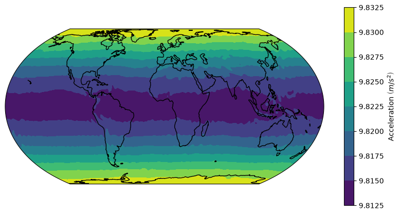
We can see how, as expected, the acceleration is highest at the poles, due to Earth’s flattening. Also, despite the fact that we are not using a high-resolution model, the Indian Ocean Geoid Low is also clearly visible.