Working with EOP data#
Added in version 7.3.0.
heyoka.py provides the ability to access Earth orientation parameters (EOP) data and use it in the expression system to represent EOP indices as time-varying quantities. This makes it possible to formulate ODEs accounting for precise information about the Earth’s orientation. With this capability, users can model dynamical systems with greater accuracy, incorporating real-world variations in the Earth’s rotation and pole position directly into their simulations.
Accessing the raw data#
The raw EOP data is encapsulated in the eop_data class. Let us explore it a bit.
import heyoka as hy

# Default-construct an eop_data instance.
data = hy.eop_data()
The raw data is available via the table property, which returns a structured NumPy array containing a time series of the EOP data:
data.table
array([(41684., 0.8075   , 0.143   , 0.137   , -18.637, -3.667),
       (41685., 0.8044   , 0.141   , 0.134   , -18.636, -3.571),
       (41686., 0.8012   , 0.139   , 0.131   , -18.669, -3.621), ...,
       (61309., 0.0073982, 0.181439, 0.312328,   0.119,  0.216),
       (61310., 0.006602 , 0.180284, 0.311707,   0.117,  0.213),
       (61311., 0.0058462, 0.179114, 0.311101,   0.114,  0.213)],
      shape=(19628,), dtype={'names': ['mjd', 'delta_ut1_utc', 'pm_x', 'pm_y', 'dX', 'dY'], 'formats': ['<f8', '<f8', '<f8', '<f8', '<f8', '<f8'], 'offsets': [0, 8, 16, 24, 32, 40], 'itemsize': 48, 'aligned': True})
The dtype of the array is eop_data_row, which contains:
the UTC MJD (
mjd),the UT1-UTC difference in seconds (
delta_ut1_utc),the \(x\) component of the polar motion in arcsecs (
pm_x),the \(y\) component of the polar motion in arcsecs (
pm_y),the \(x\) component of the correction to the IAU 2000/2006 precession/nutation model in milliarcsecs (
dX),the \(y\) component of the correction to the IAU 2000/2006 precession/nutation model in milliarcsecs (
dY).
Updating the EOP data#
A default-constructed eop_data instance uses a builtin EOP dataset from the IERS datacenter ("finals2000A.all"). This dataset is comprehensive, including both historical data dating back to the 70s and predictions for the near future.
Although the builtin dataset is updated at every new heyoka.py release, it is likely to be outdated, at least for operational uses. For this reason, the eop_data class provides static factory methods to construct eop_data instances from up-to-date datasets downloaded from the internet.
As an example, we can use fetch_latest_iers_rapid() to download the "finals2000A.daily" dataset, which contains EOP data and predictions for an interval of 180 days around the present time:
updated_data = hy.eop_data.fetch_latest_iers_rapid(filename="finals2000A.daily")
Please see the documentation of eop_data for more detailed information.
Using the EOP data in the expression system#
heyoka.py’s expression system includes several EOP quantities implemented as time-dependent functions. These EOP functions can then be employed, e.g., to formulate the dynamics of Earth-orbiting spacecraft.
The EOP functions are all implemented as piecewise linear functions of the input time coordinate, and currently they include:
the Earth rotational angle
era()and its derivative,the Greenwich mean sidereal time
gmst82()and its derivative,the polar motion angles
pm_x()andpm_y()and their derivatives,the corrections to the IAU 2000/2006 precession/nutation model
dX()anddY()and their derivatives.
All these functions take in input a time expression meant to represent the number of Julian centuries elapsed since the epoch of J2000 in the terrestrial time (TT) timescale. They also accept as a second (optional) argument the eop_data dataset to be used in the computation - if not provided, the builtin EOP dataset will be used.
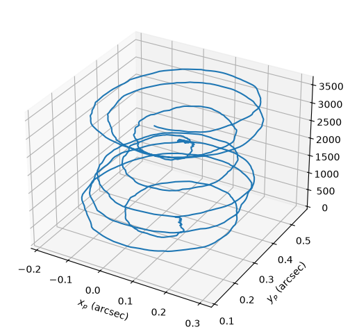
Here is an example of computation and visualisation of the time evolution of the polar motion angles using heyoka.py’s compiled functions:
import numpy as np

# Define the computation timespan: 10 years following J2000.
tspan = np.linspace(0, 0.1, 1000)

# Introduce a symbolic variable for the representation of time.
tm = hy.make_vars("tm")

# Construct a compiled function for the computation of the polar motion angles.
cf = hy.cfunc([hy.model.pm_x(time_expr=tm), hy.model.pm_y(time_expr=tm)], [tm])

# Compute the values of the polar motion angles over tspan.
pm_x, pm_y = cf(inputs=[tspan])
%matplotlib inline
from matplotlib.pylab import plt

fig = plt.figure(figsize=(6, 6))
ax = fig.add_subplot(projection="3d")

# Convert the angles to arcsec and the timespan
# to days for visualisation.
rad_to_arcsec = 180 * 3600 / np.pi
cy_to_days = 36525

ax.plot(pm_x * rad_to_arcsec, pm_y * rad_to_arcsec, tspan * cy_to_days)
ax.set_xlabel("$x_p$ (arcsec)")
ax.set_ylabel("$y_p$ (arcsec)");
Using custom EOP datasets#
Added in version 7.12.0.
In addition to the builtin and downloadable data sets, it is also possible to manually construct EOP datasets from user-supplied data.
First, we generate the raw data table as a structured NumPy array (using some invented values for the MJDs and the EOP quantities):
tbl = np.array(
    [
        (41684.0, 0.8075, 0.143, 0.137, -18.637, -3.667),
        (41685.0, 0.8044, 0.141, 0.134, -18.636, -3.571),
        (41686.0, 0.8012, 0.139, 0.131, -18.669, -3.621),
    ],
    dtype=hy.eop_data_row,
)
Then, we need to pick an identifier and a timestamp for our custom EOP dataset. heyoka.py internally uses timestamp and identifier to discriminate between EOP datasets: two datasets with the same timestamp, identifier and number of data rows are considered identical.
Both timestamp and identifier can be arbitrary strings, as long as they are non-empty and they do not contain the - or . characters:
timestamp = "20260611"
identifier = "my_custom_data"
Now we can proceed to the construction of our custom EOP dataset:
custom_data = hy.eop_data(data=tbl, timestamp=timestamp, identifier=identifier)
The custom dataset is now ready to be used in the expression system:
# Construct an expression for the x component of the polar motion
# using the custom dataset.
hy.model.pm_x(eop_data=custom_data)
eop_pm_x_3_20260611-my_custom_data(t)
As you can see, the timestamp, the identifier and the number of rows have all been mangled into the name of the function.