Atmospheric drag

In this section, we will formulate the perturbation experienced by an Earth-orbiting spacecraft due to the Earth’s atmosphere.

Theoretical background

We begin with the formula for the acceleration induced by quadratic drag on a spacecraft:

\[ \mathbf{a}_D = -\frac{1}{2}\rho v_{\mathrm{rel}} \frac{C_DA}{m} \mathbf{v}_{\mathrm{rel}}, \]

where \(\mathbf{v}_{\mathrm{rel}}\) is the velocity of the spacecraft relative to the atmosphere, \(v_{\mathrm{rel}}=\left| \mathbf{v}_{\mathrm{rel}} \right|\), \(\rho\) is the atmospheric density and \(C_D\), \(A\) and \(m\) are, respectively, the drag coefficient, cross sectional area and mass of the spacecraft. An equivalent formulation is:

\[ \mathbf{a}_D = -\frac{1}{2}\rho v_{\mathrm{rel}}C_b \mathbf{v}_{\mathrm{rel}}, \]

where \(C_b=\frac{C_DA}{m}\) is the ballistic coefficient of the spacecraft (or its inverse, depending on the convention).

The air density \(\rho\) can be calculated from a standard atmospheric model, where it is typically given as a function of the position of the spacecraft in an Earth-fixed frame, a time coordinate and solar weather indices. Here we will be using our own implementation of the NRLMSISE-00 atmospheric model, described in detail in another tutorial.

Unless otherwise noted, we will be operating in SI units, with time counted in TT seconds since J2000.

Coordinate transformations

While spacecraft dynamics is most easily formulated in a non-rotating reference frame (such as the GCRS), we will need to rotate to an Earth-fixed frame (such as the ITRS) in order to compute \(\rho\) and \(\mathbf{v}_{\mathrm{rel}}\).

We start off by introducing \(x,y,z\) as the Cartesian coordinates of the spacecraft in the GCRS:

import heyoka as hy

# Cartesian coordinates in the GCRS.
x, y, z = hy.make_vars("x", "y", "z")

The Cartesian coordinates in the ITRS \(x_{\mathrm{ITRS}},y_{\mathrm{ITRS}},z_{\mathrm{ITRS}}\) are related to \(x,y,z\) by a complex time-dependent relation (which also involves Earth orientation parameters data). The rotation can be performed via the rot_icrs_itrs() function:

# Seconds in a day.
sday = 86400.0
# Days in a century.
dcy = 36525.0

# Introduce the time variable, measuring time in seconds.
tm = hy.make_vars("tm")

# Perform the rotation.
x_itrs, y_itrs, z_itrs = hy.model.rot_icrs_itrs(
    [x, y, z], thresh=1e-3, time_expr=tm / (sday * dcy)
)

Notice how we passed tm / (sday * dcy) as the time_expr argument in rot_icrs_itrs(). The reason for this is that rot_icrs_itrs() requires in input the number of centuries elapsed since the epoch of J2000, but here we want to formulate the equations of motion in SI units. Hence, we introduce a variable tm intended to represent time in seconds, and we rescale it in order to produce an expression representing time in centuries.

Notice also how we passed a thresh argument of \(10^{-3}\): this will slightly reduce the accuracy of the rotation in order to improve computational performance. Please see the documentation of rot_icrs_itrs() for more details.

We now need to apply a further transformation in order to account for the fact that atmospheric models typically accept in input geodetic coordinates. We can accomplish this via the cart2geo() function:

h, lat, lon = hy.model.cart2geo([x_itrs, y_itrs, z_itrs])

Lastly, we need to compute \(\mathbf{v}_{\mathrm{rel}}\). In order to do this, we first introduce the variables \(v_x, v_y, v_z\) representing the spacecraft’s Cartesian velocity components in the GCRS:

vx, vy, vz = hy.make_vars("vx", "vy", "vz")

We then have to compute the atmosphere’s velocity at the spacecraft position. In order to do this, we proceed in stages.

First, under the assumption of an atmosphere co-rotating with the Earth, we introduce a point with fixed ITRS coordinates \(\left( x_0, y_0, z_0 \right)\):

x0, y0, z0 = hy.make_vars("x0", "y0", "z0")

Then, we apply an ITRS->GCRS rotation in order to calculate the point’s Cartesian position in the GCRS:

x0_gcrs, y0_gcrs, z0_gcrs = hy.model.rot_itrs_icrs(
    [x0, y0, z0], thresh=1e-3, time_expr=tm / (sday * dcy)
)

We then take the time derivative in order to produce expressions for the velocity components of the fixed point in the GCRS:

vx0_gcrs, vy0_gcrs, vz0_gcrs = hy.diff_tensors(
    [x0_gcrs, y0_gcrs, z0_gcrs], diff_args=[tm]
).jacobian.flatten()

Finally, we replace \(\left( x_0, y_0, z_0 \right)\) with \(\left( x_{\mathrm{ITRS}},y_{\mathrm{ITRS}},z_{\mathrm{ITRS}} \right)\). This will yield the atmosphere’s GCRS velocity as a function of the spacecraft’s GCRS position:

vx_atm, vy_atm, vz_atm = hy.subs(
    [vx0_gcrs, vy0_gcrs, vz0_gcrs], {x0: x_itrs, y0: y_itrs, z0: z_itrs}
)

\(\mathbf{v}_{\mathrm{rel}}\) is now easily computed as \(\mathbf{v} - \mathbf{v}_{\mathrm{atm}}\):

vrel_x, vrel_y, vrel_z = vx - vx_atm, vy - vy_atm, vz - vz_atm

The atmospheric model

As mentioned earlier, we will be using the NRLMSISE-00 atmospheric model, implemented in heyoka.py via the nrlmsise00_tn() function. In addition to the geodetic coordinates of the spacecraft, the model requires in input several space weather parameters. Please see the space weather tutorial for more information on how to manage space weather data in heyoka.py.

We begin with the definition of the time coordinate for the model. As the documentation of nrlmsise00_tn() indicates, the time coordinate is expected to represent the number of fractional days elapsed since January 1st UTC 00:00. We can use the handy dayfrac() function for this purpose:

# Time coordinate for use in the atmospheric model.
tm_atm = hy.model.dayfrac(tm / sday)

Again, we rescale tm by sday because the dayfrac() function expects an input time measured in days, while tm measures time in seconds.

Next, we introduce the space weather indices, using the f107(), f107a_center81() and Ap_avg() functions:

f107 = hy.model.f107((tm - sday) / (sday * dcy))
f107a = hy.model.f107a_center81(tm / (sday * dcy))
ap = hy.model.Ap_avg(tm / (sday * dcy))

Notice the offsetting by a day of the time coordinate passed to f107(): as indicated in the documentation of nrlmsise00_tn(), the f107 index of the day before tm must be used.

We can now assemble the expression for the air density:

rho = hy.model.nrlmsise00_tn(
    [h / 1000.0, lat, lon], f107=f107, f107a=f107a, ap=ap, time_expr=tm_atm
)

Note how we divided h by 1000: this is because we are measuring h in metres, but the nrlmsise00_tn() function requires an altitude in kilometres instead.

Assembling the dynamics

We can now proceed to the formulation of the drag-induced acceleration.

First we compute \(v_\mathrm{rel}\):

vrel = hy.sqrt(hy.sum([vrel_x**2, vrel_y**2, vrel_z**2]))

The ballistic coefficient \(C_b\) is easily introduced as a runtime parameter:

Cb = hy.par[0]

We can now assemble the expression fo the drag-induced acceleration:

import numpy as np

acc_drag = -0.5 * rho * vrel * Cb * np.array([vrel_x, vrel_y, vrel_z])

As a final step, we replace the time variable tm with the heyoka.time expression. In the previous steps, it was convenient to represent time via a regular variable (so that, e.g., we could take the time derivative in order to compute the atmospheric velocity). For use in ODE integration, however, time must be represented via the heyoka.time expression:

acc_drag = hy.subs(acc_drag, {tm: hy.time})

Visualising the drag acceleration

We can now proceed to a visual qualitative check of the computed drag acceleration.

First, we introduce a value for the ballistic coefficient of our spacecraft:

Cb_val = 0.00019366446 * 2 / 0.15696615

This value has been computed from the BSTAR coefficient of the Hubble space telescope as published on CelesTrak.

We then proceed to introduce a compiled function for the numerical computation of the drag acceleration:

cf_acc_drag = hy.cfunc(acc_drag, [x, y, z, vx, vy, vz], compact_mode=True)

As a first check, we can visualise how the drag acceleration changes with the orbital radius. For this computation, we fix the time coordinate at \(t=0\), that is, J2000:

Nsamples = 1000

# Prepare the x/y/z/vx/vy/vz inputs. We use circular equatorial orbits
# of increasing radius.
earth_mu = 3.986e14
inputs = np.zeros((6, Nsamples))
xrange = np.linspace(6.910e6, 4.2e7, Nsamples)
# Initial x coordinate.
inputs[0] = xrange
# Initial vy velocity.
inputs[4] = np.sqrt(earth_mu / xrange)

# Compute and visualise the acceleration.
acc_r = np.linalg.norm(
    cf_acc_drag(inputs, pars=[[Cb_val] * Nsamples], time=[0.0] * Nsamples), axis=0
)

%matplotlib inline
from matplotlib.pylab import plt

fig = plt.figure(figsize=(8, 4))

plt.semilogy(xrange / 1000.0, acc_r)

plt.title("Drag acceleration as a function of orbital radius")
plt.xlabel(r"Orbital radius $\left( \mathrm{km} \right)$")
plt.ylabel(r"Acceleration $\left(\mathrm{m}/\mathrm{s}^2\right)$")

plt.tight_layout()

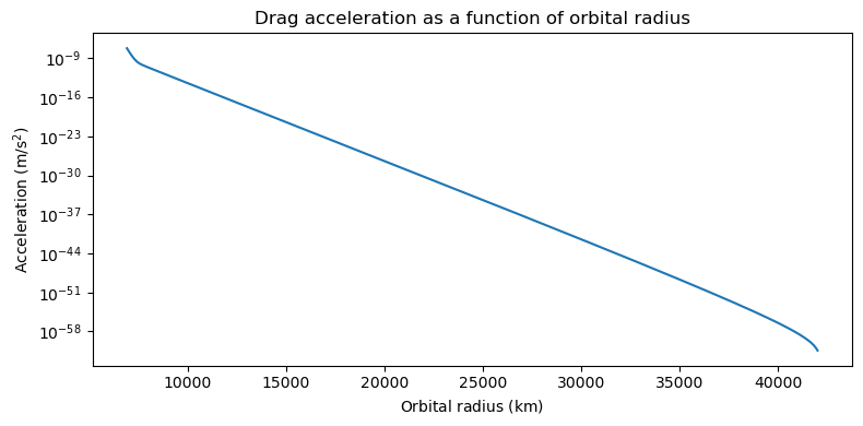
We can see how the acceleration starts at \(\sim 10^{-7}\,\mathrm{m}/\mathrm{s}^2\) in LEO, and decays exponentially as the orbital radius increases.

Next, we look at the time evolution of the drag acceleration in LEO. First we look at the evolution over 1 year starting from J2000:

inputs = np.zeros((6, Nsamples))
trange = np.linspace(0, 86400 * 365.25, Nsamples)
inputs[0] = 6.910e6
inputs[4] = np.sqrt(earth_mu / 6.910e6)

acc_hist = np.linalg.norm(
    cf_acc_drag(inputs, pars=[[Cb_val] * Nsamples], time=trange), axis=0
)

fig = plt.figure(figsize=(8, 4))

plt.semilogy(trange / 86400, acc_hist)

plt.title("Drag acceleration in LEO as a function of time")
plt.xlabel(r"Days since J2000")
plt.ylabel(r"Acceleration $\left(\mathrm{m}/\mathrm{s}^2\right)$")

plt.tight_layout()

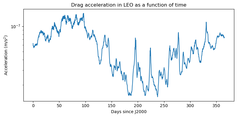
We can clearly see a noisy yearly cycle punctuated by occasional spikes due to geomagnetic storms.

We can broaden the time horizon and look at the evolution over 22 years (roughly 2 solar cycles):

trange = np.linspace(0, 86400 * 365.25 * 22, Nsamples)

acc_hist = np.linalg.norm(
    cf_acc_drag(inputs, pars=[[Cb_val] * Nsamples], time=trange), axis=0
)

fig = plt.figure(figsize=(8, 4))

plt.semilogy(trange / (86400 * 365.25), acc_hist)

plt.title("Drag acceleration in LEO as a function of time")
plt.xlabel(r"Years since J2000")
plt.ylabel(r"Acceleration $\left(\mathrm{m}/\mathrm{s}^2\right)$")

plt.tight_layout()

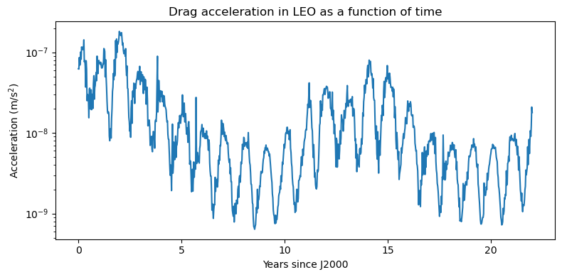
We can see again the yearly variations superimposed over the longer 11-year period of the solar cycle. Note how the drag acceleration can change by two orders of magnitude between solar maximum and solar minimum.

An example of orbital decay

In this last section, we will plug the drag acceleration into an ODE solver in order to show a concrete example of orbital decay.

In order to keep things simple, we will assume a Keplerian model for the Earth’s gravitational field. We can use the fixed_centres() function for this purpose:

# Define Keplerian dynamics.
dyn = hy.model.fixed_centres(earth_mu, [1.0], [[0.0, 0.0, 0.0]])

We can then add the drag acceleration terms:

dyn[3] = (dyn[3][0], dyn[3][1] + acc_drag[0])
dyn[4] = (dyn[4][0], dyn[4][1] + acc_drag[1])
dyn[5] = (dyn[5][0], dyn[5][1] + acc_drag[2])

In order to detect orbital decay, we will be using a terminal event, with a reentry radius of \(6491\,\mathrm{km}\):

decay_ev = hy.t_event(x**2 + y**2 + z**2 - (6.491e6) ** 2)

We can now instantiate the numerical integrator, placing our spacecraft on a Keplerian equatorial orbit at an altitude similar to the ISS:

r0 = 6.778e6
ta = hy.taylor_adaptive(
    dyn,
    [r0, 0.0, 0.0, 0.0, np.sqrt(earth_mu / r0), 0.0],
    t_events=[decay_ev],
    compact_mode=True,
    # NOTE: remember to assign the ballistic coefficient
    # to the pars array.
    pars = [Cb_val]
)

And we let it run until decay, making sure to enable continuous output so that we will be able to analyze the trajectory:

# Propagate for a long time, relying on the decay event to trigger in
# order to stop the integration.
res = ta.propagate_until(1e9, c_output=True)

We can now proceed to examine the results. First, we take a look at the time at which the reentry occurred:

print(f'Reentry time: {ta.time / 86400.} days after J2000')

Reentry time: 895.0561278122303 days after J2000

Second, we can plot the evolution of the radial coordinate of the spacecraft over time, which will give us a qualitative idea of the reentry profile:

trange = np.linspace(0, ta.time, Nsamples)

r_hist = np.linalg.norm(
    res[4](trange)[:,:3], axis=1
)

fig = plt.figure(figsize=(8, 4))

plt.plot(trange / 86400, r_hist / 1000.)

plt.title("Orbital decay in LEO")
plt.xlabel("Days since J2000")
plt.ylabel(r"Orbital radius $\left(\mathrm{km}\right)$")

plt.tight_layout()

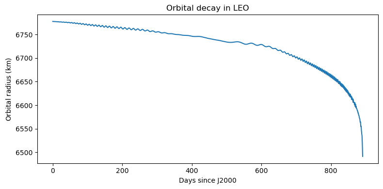
As expected, the decay of the orbital radius is gentle at first. As the atmospheric density increases, the decay rate begins to accelerate, eventually leading to a very steep profile in the final phases of the reentry.